Estimating Average Stable Periods in Hotwife Encounters

Defining Reliability: The Failure-Repair Cycle

When we manage any system that is intended to be used repeatedly, we are inherently dealing with a cycle of operation, failure, and repair. MTBF is a metric designed specifically for these repairable systems.

To understand where MTBF fits, let's look at the typical lifecycle of events for a repairable asset.

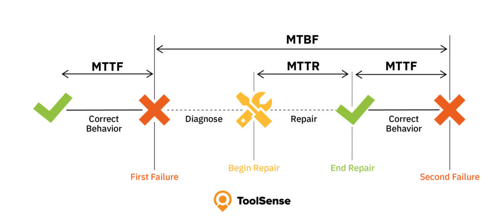
Let's clarify the terms shown in the diagram, as their usage can sometimes be ambiguous:

• Mean Time To Failure (MTTF): This represents the average time a non-repairable item is expected to function before it fails completely and is replaced (e.g., a light bulb, a battery). In diagrams like the one above, the label "MTTF" is sometimes used to denote the individual uptime periods of a repairable system.
• Mean Time To Repair (MTTR): This is the average time it takes to diagnose and repair a failure and return the system to operational status. It is a measure of maintainability.
• Mean Time Between Failures (MTBF): This is the metric we are focusing on. For a repairable system, MTBF represents the average operating time or uptime between consecutive failures.

A common point of confusion arises from diagrams where the MTBF arrow spans from one failure to the next, seemingly including the repair time. However, the standard engineering definition, and the one we will use, explicitly excludes downtime. MTBF is the average of the "Correct Behavior" periods.

To solidify this distinction, please watch the following segment.

Calculating MTBF

The calculation for MTBF is straightforward, but its accuracy depends entirely on using the correct inputs.

As you've read, the formula is:

The key is to exclude planned downtime (like scheduled maintenance) from the operating time and to only count unexpected breakdowns as failures.

Let's apply this to our two scenarios.

Application 1: Wardrobe Malfunctions in a Boudoir Photoshoot

Imagine you want to assess the reliability of your curated lingerie wardrobe. You track its performance over the last 15 photoshoots.

• Data:

  • Total duration of active shooting time across all 15 shoots: 60 hours.
  • During this time, you recorded 3 wardrobe malfunctions requiring a pause to fix or replace an item (e.g., a strap breaks, a zipper gets stuck). These are your unexpected failures.
  • You also had 5 hours of planned downtime for scheduled outfit changes, which are not failures.

• Calculation:

  • Total Operating Time: 60 hours (The planned downtime is already excluded from this "active shooting time" figure).
  • Number of Failures: 3.
  • MTBF = 60 hours / 3 failures = 20 hours.

• Interpretation:
  You can expect a wardrobe malfunction, on average, for every 20 hours of active shooting. This metric gives you a baseline. If you invest in higher-quality pieces or implement a pre-shoot inspection routine (as suggested in our FMEA lesson), you can track this MTBF value over the next set of shoots to see if your interventions are improving reliability.

Application 2: Scheduling Conflicts in the Hotwife's Encounters

Here, the "system" is the process of scheduling and executing intimate encounters, and a "failure" is a last-minute scheduling conflict that causes a cancellation. You want to measure the stability of this process from the hotwife's perspective.

• Data:

  • Observation period: 6 months (182 days).
  • During this period, 4 encounters were cancelled at the last minute due to unforeseen scheduling conflicts (e.g., bull had to work late, hotwife forgot a prior commitment).
  • You estimate that the emotional and logistical disruption from each cancellation renders the "system" effectively down for 2 days while things are smoothed over and replanned.

• Calculation:

  • Total Time: 182 days.
  • Total Downtime: 4 failures × 2 days/failure = 8 days.
  • Total Operating Time: 182 days - 8 days = 174 days.
  • Number of Failures: 4.
  • MTBF = 174 days / 4 failures = 43.5 days.

• Interpretation:
  On average, the arrangement remains stable for about 43.5 days between disruptive scheduling conflicts. This value serves as a critical performance indicator. If the involved parties implement a more robust scheduling system (e.g., a shared digital calendar), they can monitor the MTBF to quantitatively measure whether the stability of their arrangement is improving.

The Statistical Foundation: MTBF and the Poisson Process

Given your background in statistics and stochastic processes, you'll recognize that the MTBF calculation rests on a powerful theoretical foundation. The so-called "classical MTBF test" assumes that failures are independent events that occur at a constant average rate. This describes a Homogeneous Poisson Process (HPP).

In an HPP, the number of events (failures) in a given interval follows a Poisson distribution, and the time between those events follows an exponential distribution. The rate parameter of this process, $\lambda$ (lambda), is the failure rate.

You can see immediately that MTBF is simply the reciprocal of the failure rate:

This inverse relationship is the core connection between the observed frequency of failures and the average time you can expect to wait for one.

The following video provides an excellent example of this relationship in action.

A key implication of modeling failure times with an exponential distribution is its memoryless property. This means that the probability of a system failing in the next hour is constant, regardless of how many hours it has already operated successfully. The system doesn't "age" or "get tired." This is a strong assumption and a key point of interpretation. While it holds well for complex systems with many components where failures appear random, it may not hold for single components subject to wear and tear. We will address those cases with Weibull analysis in a later lesson.

Conclusion

In this lesson, we have added a powerful quantitative tool to your reliability toolkit. Moving beyond the qualitative risk assessment of FMEA, you can now calculate and interpret MTBF to measure the actual, observed reliability of a system.

Key Takeaways:

• MTBF quantifies reliability: It measures the average uptime between failures for repairable systems.
• Calculation requires careful data selection: MTBF is calculated as Total Operating Time / Number of Failures, where only unexpected failures and actual uptime are included.
• MTBF has a strong statistical basis: It is the reciprocal of the constant failure rate ($\lambda$) in a Homogeneous Poisson Process, where the time between failures is exponentially distributed.
• Interpretation is key: MTBF provides a baseline for measuring performance and the effectiveness of reliability improvements. Understanding the underlying "constant failure rate" assumption is crucial for its proper application.

You now have a way to answer "How often do things go wrong?". With this knowledge, a natural next question is "What can we do to make our system tolerate these failures?". In our next lesson, we will explore Redundancy Optimization, a primary strategy for designing resilience and improving the overall reliability of a system, particularly when its MTBF is lower than desired.