Weibull Analysis of Hotwife Outfits & Encounter Stressors

The "Weakest Link" and the Nature of Failure

Many systems fail not because everything wears out at once, but because a single critical component—the weakest link—gives way. A lingerie outfit might become unusable because one strap snaps; a period of high relationship satisfaction might end because one specific unresolved issue comes to a head.

The Weibull distribution is theoretically grounded in this "weakest link" principle, which is a result from Extreme Value Theory. Given your background in statistics, you'll recognize this as analogous to how the Central Limit Theorem motivates the Normal distribution for sums of random variables. Here, Extreme Value Theory shows that the distribution of the minimum of many random variables (i.e., the time until the first component fails) often converges to a Weibull distribution.

For a deeper look into this theoretical justification and the formal definition of the Weibull distribution, the following resource is excellent.

As you've read, the 2-parameter Weibull distribution is defined by:

1. Scale parameter ($\alpha$), or Characteristic Life: This parameter represents the time at which approximately 63.2% of the population will have failed. It stretches or compresses the distribution along the time axis.
2. Shape parameter ($\beta$), or Weibull Modulus: This is the most insightful parameter. It describes the nature of the failure pattern over time.

Interpreting the Shape Parameter: The Bathtub Curve

The value of the shape parameter, $\beta$, tells a story about how the failure rate evolves. This is often visualized using the "Reliability Bathtub Curve."

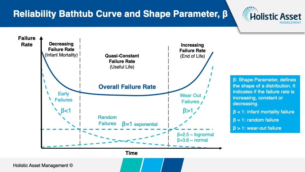
The three phases are:

• $\beta <1$: Decreasing Failure Rate (Infant Mortality). Failures are more likely at the beginning of life, often due to manufacturing defects or initial setup problems. As these faulty units are weeded out, the failure rate for the remaining population decreases.
• $\beta =1$: Constant Failure Rate (Random Failures). The failure rate is constant over time. A failure is just as likely to happen now as it is a year from now, regardless of age. This corresponds to the exponential distribution, which was the implicit model in our previous lessons on MTBF and redundancy. These failures are typically caused by random external events or shocks.
• $\beta >1$: Increasing Failure Rate (Wear-Out). The failure rate increases with time. This is the classic aging effect, where components degrade, fatigue, and become more susceptible to failure as they accumulate use.

The shape parameter dramatically alters the form of the probability density function, as shown below. A high $\beta$ leads to a tight, predictable distribution of failures, while a low $\beta$ indicates a wide, skewed distribution with many early failures.

To formalize this, we use the hazard function, $h(t)$, which gives the instantaneous probability of failure at time $t$, given that the unit has survived up to time $t$. For the Weibull distribution, the hazard function is $h(t)=\frac{\beta }{\alpha }(\frac{t}{\alpha }{)}^{\beta -1}$. You can see directly from this formula how the value of $\beta$ determines whether the hazard rate decreases, is constant, or increases with time $t$.

From Data to Insight: A Practical Walkthrough

Theory is powerful, but how do we apply it? Imagine you've collected data on when items fail. How do you estimate $\alpha$ and $\beta$ and use them to make predictions?

The video below provides a superb, step-by-step practical guide using a method that linearizes the Weibull CDF. By taking the natural logarithm twice, we can transform the equation into the form of a line, $y=mx+b$, making it easy to fit to data and extract the parameters.

Let's apply this process to our scenarios.

Application 1: Modeling Photoshoot Outfit Failure

Suppose you want to understand the reliability of a particular style of lingerie used in photoshoots. You track 20 identical pieces and record the number of uses (shoots) until each one "fails"—meaning it's no longer usable due to wear, tear, or loss of aesthetic quality.

1. Collect Data: You have a list of 20 failure times (e.g., 15 uses, 22 uses, 18 uses...).
2. Rank and Plot: Following the video's method, you would:
   • Sort the failure times from lowest to highest.
   • Assign a rank $i$ from 1 to 20.
   • Calculate the cumulative failure probability for each, $F=(i-0.5)/20$.
   • Calculate the Y-axis values: $\ln (\ln (1/(1-F)))$.
   • Calculate the X-axis values: $\ln (\text{uses to failure})$.
   • Create a scatter plot of Y vs. X and fit a linear trendline.
3. Interpret the Results: The trendline equation will be in the form $y=mx+b$.
   • The slope, $m$, is your estimate for the shape parameter, $\hat{\beta }$. If $\hat{\beta }>1$ (e.g., 2.5), it confirms that the outfits are failing due to wear-out, which is expected.
   • From the slope ($\hat{\beta }$) and intercept ($b=-\hat{\beta }\ln (\hat{\alpha })$), you can solve for the characteristic life, $\hat{\alpha }$. This tells you the number of uses by which 63.2% of your outfits will have failed.
4. Make Predictions: With your model ($y=\hat{\beta }x-\hat{\beta }\ln (\hat{\alpha })$), you can now answer critical questions, as demonstrated in the video:
   • "What is the number of uses below which we can expect only a 1% failure rate?" You set F=0.01, calculate the corresponding $y$ value, and solve for $x=\ln (\text{uses})$.
   • "After 50 uses, what is the expected probability of an outfit having failed?" You set uses=50, calculate $x=\ln (50)$, solve for $y$, and then reverse the transformation to find $F$.

Application 2: Analyzing the Timing of Relationship Stressors

This application is more abstract but follows the same logic. Let's define a "failure" as a significant stress event that disrupts the intimacy between the hotwife and her bull. The "time to failure" is the duration (in weeks or months) between these events.

1. Collect Data: You have a log of the time between these stress events over a long period (e.g., 12 weeks, 20 weeks, 8 weeks...).
2. Rank and Plot: You perform the same Weibull analysis as above on these time-between-event durations.
3. Interpret the Results: The estimated shape parameter, $\hat{\beta }$, provides deep insight into the relationship's dynamics:
   • $\hat{\beta }>1$ (Wear-out): Stressors are becoming more frequent over time. This is a critical warning sign, suggesting that minor unresolved issues are accumulating or that the relationship is experiencing fatigue. The system is degrading.
   • $\hat{\beta }=1$ (Random): Stressors occur at a constant rate, likely triggered by unpredictable external factors rather than an internal dynamic. The relationship itself is stable in its response to shocks.
   • $\hat{\beta }<1$ (Infant Mortality): Stressors were more frequent at the beginning but have become less frequent over time. This is a positive sign, indicating that the partners have learned, adapted, and built a more resilient system for handling conflict.

A Note on Estimation

The graphical method using Excel is powerful for building intuition. As a statistician, you know that more robust methods are preferred for formal analysis. The standard approach is Maximum Likelihood Estimation (MLE), which finds the parameter values that maximize the probability of observing the data you actually collected. These methods are computationally intensive but are standard in statistical software.

The tutorial by Scholz provides a rigorous overview of MLE for the Weibull distribution and its implementation in R.

An important real-world consideration is censored data—for instance, when your study ends, some outfits may still be in perfect condition. We know their lifetime is at least a certain value, but we don't know the exact failure time. MLE methods are particularly well-suited to correctly incorporate this type of incomplete information.

Conclusion

Today, we've added a crucial tool to our reliability toolkit. By moving from a simple constant failure rate to the flexible Weibull distribution, we can now model a wide range of real-world failure behaviors.

Key Takeaways:

• The Weibull distribution is a powerful model for time-to-failure analysis, theoretically grounded in the "weakest link" principle.
• The shape parameter ($\beta$) is the key to interpretation, revealing whether a system exhibits infant mortality ($\beta <1$), random failures ($\beta =1$), or wear-out ($\beta >1$).
• By fitting a Weibull distribution to failure data, we can estimate its parameters and build a predictive model to quantify risk and reliability. This can be done graphically or with more statistically robust methods like MLE.
• This analysis provides deep insights, whether modeling the physical wear of a lingerie piece or the abstract timing of stressors in a relationship.

In our next lesson, we will put this knowledge to immediate use. Understanding the failure pattern—specifically, whether failure is sudden and random or gradual and predictable—is the first step in designing an intelligent replacement strategy. We will explore how to use our $\beta$ estimate to decide when and how to replace assets, from photoshoot wardrobe items to relationship agreements.