Calculating Implied Volatility from Option Prices

Introduction

In our previous lessons, we've treated volatility ( $σ$ ) as a known input to the Black-Scholes-Merton (BSM) formula. We took the stock price, strike, time, risk-free rate, and volatility to compute an option's theoretical price. Today, we turn this logic on its head. In the real world, option prices are set by supply and demand in the market. The one piece of the BSM puzzle that isn't directly observable is the future volatility of the underlying asset.

This lesson explores how we can use the observable market price of an option to work backward and solve for the volatility that the market is "implying." This crucial metric, known as implied volatility (IV), represents the market's collective consensus on the likely magnitude of future price swings. By the end of this lesson, you will be able to explain the process of calculating implied volatility from a market price, a fundamental skill in both option trading and risk management.

What is Implied Volatility?

At its core, implied volatility is the value of $σ$ that makes the BSM model price equal to the option's currently traded market price. All other inputs—stock price ( $S$ ), strike price ( $K$ ), time to maturity ( $T$ ), and risk-free rate ( $r$ )—are known.

This short video provides an excellent conceptual starting point.

Option Implied Volatility Explained + How to Calculate It in Excel

The video "Option Implied Volatility Explained" by Ryan O'Connell, CFA, FRM, clearly introduces the concept.

Watch the first segment from the beginning until the Excel part. The speaker effectively lists the BSM inputs and highlights that volatility is the only one that isn't directly observable. He explains that we use the observed option price to solve for this unknown volatility.

The problem we need to solve is finding the specific value $σ_{I V}$ that satisfies the following equation:

\text{BSM_Price}(S, K, T, r, \sigma_{IV}) = \text{Market_Price}

A critical property of the BSM model makes this possible: the price of a European option is a strictly increasing, continuous function of volatility. This means that for any valid market price, there is one and only one corresponding implied volatility. This uniqueness guarantees that the problem is well-posed.

The Challenge: Inverting the BSM Formula

Unfortunately, the BSM formula is a complex mix of logarithms, exponentials, and the cumulative normal distribution function. There is no algebraic way to rearrange the equation to solve for $σ$ directly.

Therefore, we must turn to numerical methods. The task is reframed as a root-finding problem. We define a function, let's call it $f (σ)$ , which represents the difference between the BSM price and the market price:

f(\sigma) = \text{BSM_Price}(\sigma) - \text{Market_Price}

Our goal is to find the value of $σ$ for which $f (σ) = 0$ . This is a common task in numerical analysis, and one of the most efficient algorithms for it is the Newton-Raphson method.

The Newton-Raphson Method

The Newton-Raphson method is an iterative algorithm that uses a function's derivative to find its root with remarkable speed. The intuition is to start with an initial guess, approximate the function with its tangent line at that point, and find where the tangent line crosses the x-axis. This crossing point becomes our next, better guess.

The general update formula for an iteration is:

σ_{n + 1} = σ_{n} - \frac{f ( σ _{n} )}{f ^{'} ( σ _{n} )}

Where:

$σ_{n}$ is our current guess for volatility.
$σ_{n + 1}$ is our next, improved guess.
$f (σ_{n})$ is the value of our function (the pricing error) at the current guess.
$f^{'} (σ_{n})$ is the derivative of the function with respect to $σ$ at the current guess.

For our specific problem, $f(\sigma) = \text{BSM_Price}(\sigma) - \text{Market_Price}$ . The derivative, $f^{'} (σ)$ , is simply the derivative of the BSM price with respect to volatility, since the market price is a constant. You may recognize this derivative from our upcoming discussion on the "Greeks"—it is Vega ( $V$ ).

Substituting these into the formula gives us the specific iterative process for finding implied volatility:

\sigma_{n+1} = \sigma_n - \frac{\text{BSM_Price}(\sigma_n) - \text{Market_Price}}{\text{Vega}(\sigma_n)}

The following resource provides a detailed explanation of this method.

Implied Volatility and Volatility Smile: Computing IV in Python ...

This article from mbrenndoerfer.com, "Implied Volatility and Volatility Smile," offers a clear breakdown of the numerical methods involved.

Please read the section titled "Computing Implied Volatility". Pay close attention to how the general root-finding problem is set up and how the Newton-Raphson update formula is derived, specifically noting the substitution of Vega as the derivative.

The iterative process is as follows:

Initialize: Start with an initial guess, $σ_{0}$ (e.g., 0.25).
Iterate: For a set number of iterations or until convergence:
a. Calculate the BSM price and Vega using the current volatility guess, $σ_{n}$ .
b. Calculate the pricing error: BSM_Price - Market_Price.
c. If the absolute error is below a defined tolerance (e.g., 0.0001), stop. $σ_{n}$ is our answer.
d. Update the volatility guess using the Newton-Raphson formula: $σ_{n + 1} = σ_{n} - \frac{Error}{Vega}$ .
Result: The final value of $σ$ is the implied volatility.

This next video demonstrates the implementation of this iterative loop in Python, which can help visualize the algorithm's steps.

Option Implied Volatility using Newton's Method in Python

The video "Option Implied Volatility using Newton's Method in Python" by QuantPy provides a practical coding perspective.

First, watch the introductory segment from the beginning. It sets up the problem and visually represents the Newton-Raphson formula in the context of implied volatility and Vega. Then, skip to the main loop of the function from the iterative process. You don't need to be a Python programmer to follow the logic: it calculates the price (bs_price), the pricing difference (c), the derivative (c_prime, which is Vega), and then updates the volatility guess (vol_new = vol_old - c / c_prime).

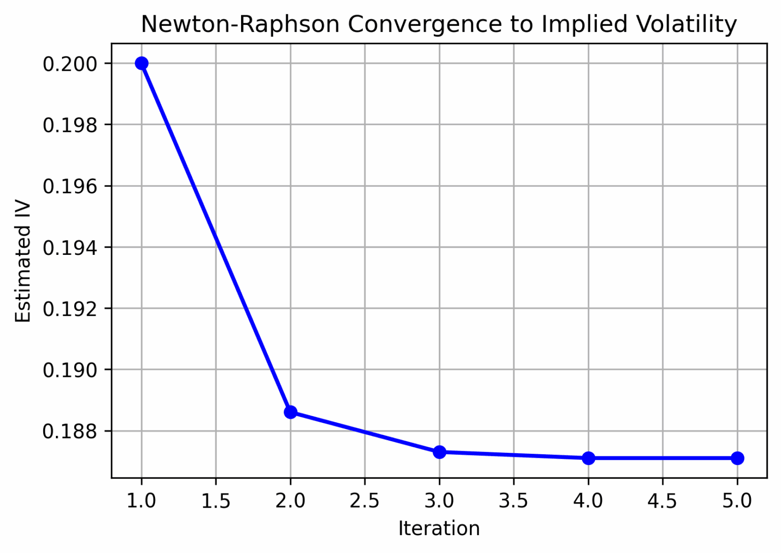
The method converges very quickly, often finding a highly accurate solution in just 3 to 5 iterations.

This chart illustrates the rapid convergence of the Newton-Raphson method. Starting from an initial guess of 20%, the estimated implied volatility quickly settles to its true value (around 18.7%) within just a few iterations.

A Worked Example: The First Iteration

Let's see how the first step works with a concrete example.

Market Data:
- Stock Price ( $S$ ): $100
- Strike Price ( $K$ ): $105
- Time to Maturity ( $T$ ): 0.5 years
- Risk-free Rate ( $r$ ): 5%
- Observed Market Price of Call: $5.50

Let's start with an initial guess of $σ_{0} = 0.20$ (or 20%).

Step 1: Calculate BSM Price and Vega at $σ_{0} = 0.20$
First, we calculate $d_{1}$ and $d_{2}$ :
$d_{1} = \frac{l n ( 100/105 ) + ( 0.05 + 0.5 \cdot 0.2 0 ^{2} ) \cdot 0.5}{0.20 0.5} \approx - 0.1018$
$d_{2} = d_{1} - 0.20 0.5 \approx - 0.2432$

Using a standard normal calculator:

$N (d_{1}) = N (- 0.1018) \approx 0.4595$
$N (d_{2}) = N (- 0.2432) \approx 0.4039$
$n (d_{1}) = \frac{1}{2 π} e^{- d_{1}^{2} /2} \approx 0.3969$

Now, calculate the BSM price and Vega:
$\text{BSM_Price}(\sigma_0) = 100 \cdot (0.4595) - 105 e^{-0.05 \cdot 0.5} \cdot (0.4039) \approx \$4.68$
$Vega (σ_{0}) = S T n (d_{1}) = 100 \cdot 0.5 \cdot (0.3969) \approx $28.06$

Step 2: Calculate the Pricing Error
$\text{Error} = \text{BSM_Price} - \text{Market_Price} = \$4.68 - \$5.50 = -\$0.82$

Step 3: Update the Volatility Guess
$σ_{1} = σ_{0} - \frac{Error}{Vega} = 0.20 - \frac{- 0.82}{28.06} = 0.20 + 0.0292 = 0.2292$

Our new, improved guess for the implied volatility is 22.92%. We would now repeat this process with $σ_{1} = 0.2292$ . After a few more iterations, the value would converge to the correct implied volatility of approximately 24.5%.

The spreadsheet below shows what a finished calculation might look like, where the "Back-solved Option Value" perfectly matches the input "Option Value" after the implied volatility has been found.

An example of an implied volatility calculator. The user provides the option's market value and other parameters, and the tool uses a numerical method to find the Implied Volatility that makes the theoretical BSM price match the market price.

Conclusion

In this lesson, we have demystified the concept of implied volatility. While it sounds complex, it is simply the missing piece of the BSM puzzle that we solve for using the observable market price.

Key Takeaways:

Implied Volatility (IV) is the market's expectation of future volatility, derived by "inverting" the BSM formula to match the observed market price of an option.
Because the BSM formula cannot be solved for volatility algebraically, we must use numerical root-finding methods.
The most common method is Newton-Raphson, an iterative algorithm that converges rapidly to the correct IV.
The core of the Newton-Raphson update step for IV is the formula $σ_{n + 1} = σ_{n} - (Pricing Error / Vega)$ .

We have assumed throughout our discussion of BSM that volatility is a single, constant number. But what happens if we calculate the implied volatility for options on the same stock, but with different strike prices? We will explore this question in our next lesson and uncover a famous pattern known as the volatility smile, a key piece of evidence highlighting the limitations of the classic BSM model.