BSM Model Limitations & the Volatility Smile

The Theory vs. The Reality

The BSM model is built on a set of simplifying assumptions. One of the most critical is that the volatility ($\sigma$) of the underlying asset's returns is constant over the life of the option and is the same for all options on that asset. If this were true, a graph of implied volatility versus strike price would be a flat, horizontal line.

However, when traders and analysts perform this exercise using real market data, they observe a distinct, predictable pattern—not a flat line.

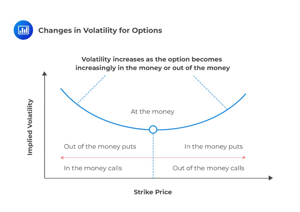
This U-shaped curve is known as the volatility smile. For some markets, particularly equity markets, the smile is not symmetrical. It often looks more like a "smirk" or a "skew," where implied volatility is highest for low strike prices (out-of-the-money puts) and decreases as the strike price rises.

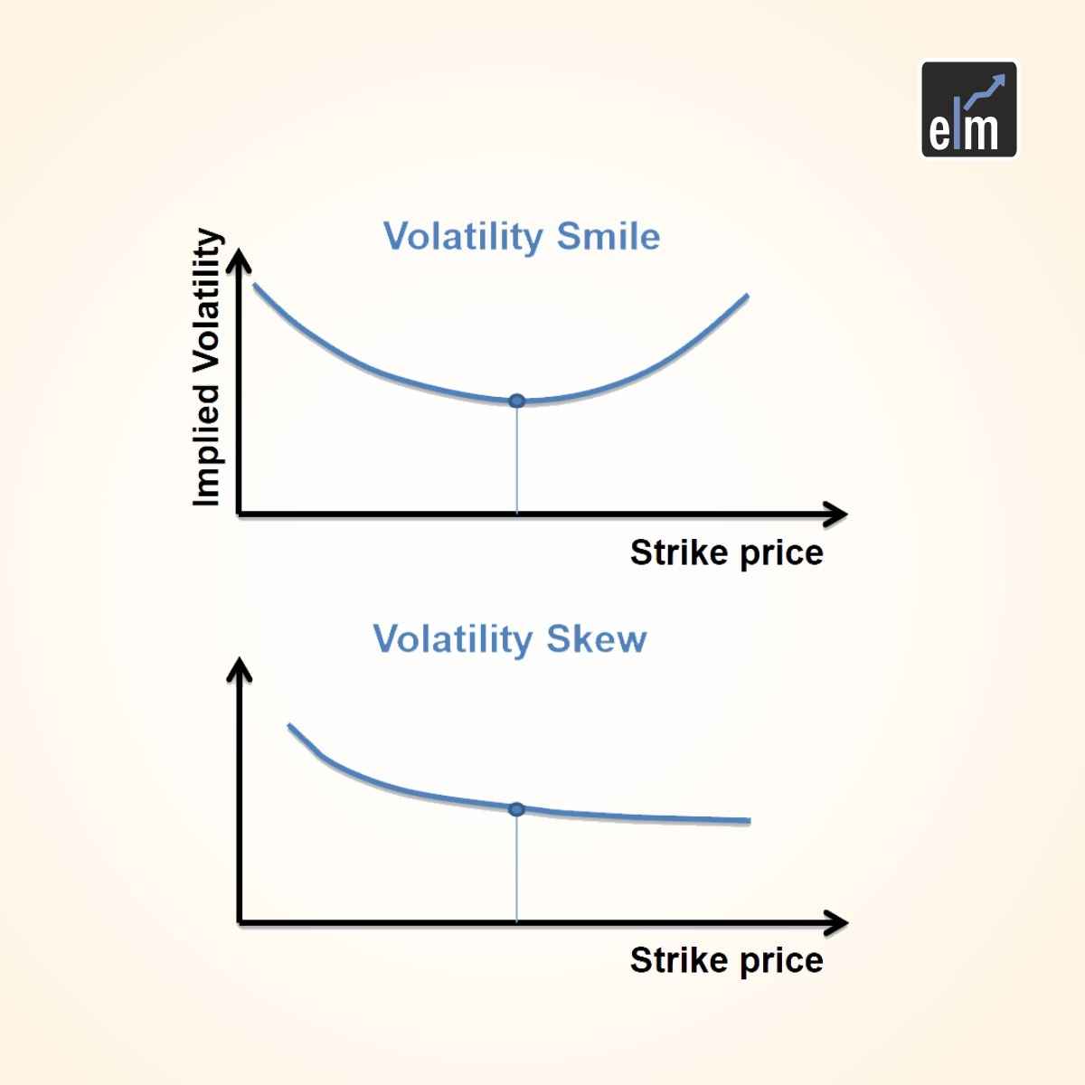
The existence of these patterns is powerful empirical evidence that the BSM model's assumptions do not perfectly capture market reality.

Why the Smile and Skew Exist: Challenging BSM's Assumptions

The volatility smile and skew are not random noise; they are the market's way of correcting for the BSM model's flawed assumptions. Given your background in statistics, you'll find the primary reasons are rooted in probability theory.

The BSM model assumes that stock prices follow a geometric Brownian motion, which implies that continuously compounded returns are normally distributed. This, in turn, means that future stock prices follow a lognormal distribution. A key feature of the normal/lognormal distribution is that extreme events are considered exceptionally rare—the distribution has "thin tails."

The following video provides a great conceptual bridge between the model's statistical underpinnings and the observed market phenomena.

As the video explains, real-world asset returns do not conform to this neat picture. Two key statistical properties are at play:

1. Fat Tails (Excess Kurtosis): Financial markets experience extreme price moves (crashes and booms) far more frequently than a lognormal distribution would predict. The distribution of actual returns has "fatter tails." The volatility smile reflects this. Traders price in a higher probability of large price moves in either direction. This increases demand for deep out-of-the-money (OTM) puts and calls, which act as insurance against these tail events, thus driving up their implied volatility.

2. Negative Skewness: For equity markets in particular, large negative returns are more common and more feared than large positive returns of the same magnitude. The distribution of equity returns is said to have a "negative skew" or a fatter left tail. This is the primary driver of the volatility skew (or smirk). Investors have a persistent demand for downside protection (e.g., portfolio insurance), which they buy in the form of OTM puts. This high demand increases the price of OTM puts, leading to higher implied volatility at lower strike prices.

The following reading provides a detailed breakdown of these drivers.

The 1987 Crash: A Permanent Shift

As noted in the reading, the volatility skew in equity markets became much more pronounced after the "Black Monday" stock market crash of October 19, 1987, when the S&P 500 fell by over 20% in a single day. According to the BSM model's lognormal assumption, such an event was statistically almost impossible. This event forced a permanent repricing of risk in the options market. Before 1987, the implied volatility curve was much flatter. Afterward, the market began persistently pricing in a higher premium for downside protection, creating the skew we see today.

This next video reinforces this historical context and explicitly links the statistical concepts of kurtosis and skewness to the smile and smirk patterns.

Other Limitations of the BSM Model

While the volatility smile is arguably the most famous limitation, the BSM model's elegance comes at the cost of several other simplifying assumptions that don't hold in practice.

Here is a summary of the key limitations discussed in the article and beyond:

• Constant Volatility and Interest Rates: The model assumes $\sigma$ and the risk-free rate $r$ are constant. In reality, both change over time. Volatility is known to cluster (periods of high volatility followed by more high volatility), and interest rates vary with maturity (the yield curve is not flat).
• Lognormal Price Distribution: As we've discussed, this is the main cause of the volatility smile. It underestimates the probability of large price jumps (fat tails/kurtosis) and ignores asymmetries (skewness).
• Continuous Trading and No Transaction Costs: The model's derivation relies on the ability to form a riskless, continuously rebalanced portfolio. Real-world trading is discrete and involves transaction costs (bid-ask spreads, commissions), making perfect, costless replication impossible.
• No Dividends: The original formula applies to non-dividend-paying stocks. While a simple adjustment (the Merton model) exists to handle a continuous dividend yield, handling discrete dividend payments is more complex.
• European-Style Options: The BSM formula is designed for European options, which can only be exercised at expiration. It cannot directly price American options, where the possibility of early exercise adds another layer of complexity.

Conclusion

In this lesson, we confronted the limitations of the elegant Black-Scholes-Merton model. While it provides a foundational framework for options pricing, its assumptions are not a perfect reflection of reality.

Key Takeaways:

• The BSM model's assumption of constant volatility across all strike prices is violated in practice.
• Plotting implied volatility against strike price reveals patterns known as the volatility smile (U-shaped) and volatility skew (downward-sloping).
• These patterns exist because the BSM model's assumption of a lognormal distribution for asset prices is flawed. Real-world returns exhibit fat tails (kurtosis) and negative skewness, which the market prices into options, especially those far from the current price.
• The volatility smile and skew are the most prominent, but other BSM limitations include the assumptions of constant interest rates, continuous trading without costs, and applicability only to European options.

Understanding these limitations is not just an academic exercise; it's essential for properly interpreting market prices and managing risk. We've now seen how option prices are sensitive to inputs like the underlying price and volatility. In the next module, we will formalize this by studying the "Greeks"—the essential risk management metrics that measure an option's sensitivity to changes in all its pricing inputs.