Assumptions of the Black-Scholes-Merton Model

Why Models Need Assumptions

Before diving into the list of assumptions, it's worth asking why we need them at all. Financial markets are incredibly complex systems. A model that tried to capture every nuance would be as complex as the market itself and therefore useless. Like a map, a good model simplifies reality to highlight the most important features for a specific task—in this case, pricing an option.

The BSM model provides this "map" by creating an idealized, frictionless world where a derivative's price can be determined with mathematical precision. To build this world, Fischer Black, Myron Scholes, and Robert Merton established a specific set of rules, which we can group into three categories: assumptions about the underlying asset, the market, and the option itself.

The BSM Assumptions

Let's begin with a high-level overview of the assumptions before breaking them down.

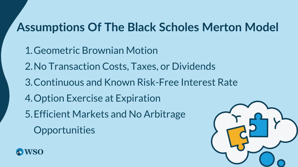
This image provides a concise list, which we will now explore in detail.

1. Assumptions about the Underlying Asset

This group of assumptions defines how the stock price is expected to behave over time.

• Random Walk: The model assumes that stock price movements follow a "random walk," specifically a Geometric Brownian Motion (GBM). You'll recognize the underlying Wiener process from your study of stochastic calculus. The SDE for the stock price $S_t$ is given by:

  $$\frac{d{S}_t}{S_t}=\mu dt+\sigma d{W}_t$$

  Here, $\mu$ is the constant expected rate of return (the drift), $\sigma$ is the constant volatility, and $d{W}_t$ is the random component from a Wiener process. This implies that stock returns are normally distributed, and consequently, stock prices are log-normally distributed. This is a key feature, as it ensures prices cannot become negative.

• Constant Volatility ($\sigma$): The model assumes the volatility of the underlying asset is constant and known throughout the option's life. This is one of the most significant simplifications, as in reality, volatility changes over time and is not known in advance. We will see later that discrepancies between this assumption and reality give rise to phenomena like the "volatility smile."

• No Dividends: The original Black-Scholes model assumes the underlying stock pays no dividends. Dividends complicate pricing because they cause predictable drops in the stock price, benefiting put holders and harming call holders. Robert Merton later extended the model to account for continuous dividend yields, which is why the model is often called Black-Scholes-Merton.

For a more detailed explanation of these points and their real-world validity, the following resource is excellent.

2. Assumptions about the Market

These assumptions create an idealized, "frictionless" market environment.

• Constant and Known Risk-Free Rate ($r$): The model assumes a single, constant risk-free interest rate at which participants can both borrow and lend any amount of money. In reality, borrowing rates are higher than lending rates, and rates change over time. However, since option prices are less sensitive to interest rates than to volatility, this assumption is often considered less problematic.

• No Transaction Costs or Taxes: All trading is assumed to be cost-free. There are no commissions, fees, or bid-ask spreads. This is the "frictionless" market assumption.

• Perfect Liquidity and Continuous Trading: The market is assumed to be perfectly liquid, meaning any quantity of the asset can be bought or sold at any time without affecting the price. Furthermore, trading can occur continuously. This is a mathematical necessity for the continuous portfolio adjustments that underpin the model's derivation, which we will explore in our next lesson.

• No Arbitrage Opportunities: This is the foundational economic principle of the model. It assumes the market is perfectly efficient, immediately eliminating any opportunity for risk-free profit. This no-arbitrage condition is what allows for pricing by replication.

Let's return to the Macroption article to explore these market assumptions.

3. Assumption about the Option

Finally, there is a crucial assumption about the type of option being priced.

• European-Style Exercise: The original BSM model is designed exclusively for European options, which can only be exercised at their expiration date. This greatly simplifies the problem by removing the need to determine the optimal time for early exercise, a complication we had to handle when pricing American options on a binomial tree. While the model is sometimes used as an approximation for American options, it can be inaccurate, especially for dividend-paying calls and deep-in-the-money puts.

Conclusion

In this lesson, we have laid out the idealized framework within which the Black-Scholes-Merton model operates. While none of these assumptions hold perfectly in the real world, they work together to create a mathematically tractable model that provides a powerful benchmark for option pricing.

Key Takeaways:

• Asset Behavior: The BSM model assumes stock prices follow a Geometric Brownian Motion with constant drift and volatility, leading to log-normally distributed prices. It also assumes no dividends are paid.
• Market Environment: The model posits a "frictionless" market with no transaction costs, a single constant risk-free rate, continuous trading, and no arbitrage opportunities.
• Option Type: The model is specifically designed to price European-style options, which can only be exercised at expiration.
• Model vs. Reality: Recognizing the discrepancy between these assumptions and the real world is the first step toward understanding the model's limitations and the purpose of more advanced derivative pricing models that relax these strict conditions.

These assumptions are not just a list to be memorized; they are the building blocks of the model's derivation. In our next lesson, we will see precisely how the assumptions of continuous trading and no-arbitrage are used to construct a continuously rebalanced, risk-free portfolio. The dynamics of this portfolio will lead us directly to the famous Black-Scholes partial differential equation (PDE), the mathematical heart of the model.