Portfolio Optimization: Constrained and Unconstrained

Introduction

In our last lesson, we explored the Tobin Separation Theorem, which elegantly simplifies portfolio construction into two distinct steps: identifying a single, optimal risky portfolio (the tangency portfolio) and then deciding how to mix it with a risk-free asset based on personal risk preference. This theory assumes we can build that tangency portfolio without any restrictions.

Today, we confront a crucial real-world complication: constraints. The most common of these is a prohibition on short-selling. This lesson will equip you to solve portfolio optimization problems when such constraints are in place. You will learn how these restrictions alter the problem and how to use numerical methods to find the optimal constrained portfolios. Mastering this is a highly practical skill for solving the numerical problems you'll face in the CM2 exam.

1. Understanding Short-Selling and Its Constraints

Before we dive into the math, let's clarify what we mean by short-selling and why it's often restricted. Short-selling is the practice of selling an asset you don't own. You borrow it from a broker, sell it on the market, and hope to buy it back later at a lower price to return to the broker, pocketing the difference. In a portfolio context, this corresponds to a negative weight for an asset.

While powerful, this strategy is not always available or advisable.

Regulatory Prohibitions: Certain investment vehicles, like pension funds or mutual funds, are often legally barred from short-selling.
Risk and Margin: Short-selling involves leverage and carries the risk of theoretically infinite losses if the asset price rises instead of falls. To mitigate this, brokers require you to post collateral, known as margin, which ties up capital and makes the process more complex than simple buying and selling.

The following video discusses the practical realities of short-selling in portfolio optimization, including the unrealistic portfolio allocations that can result without constraints and the role of margin requirements.

Portfolio management with short-selling and margining (Excel)

This video from NEDL provides a practical look at the issues surrounding short-selling in portfolio management.

Please watch the following segments: Introduction (from the start): The presenter explains why unconstrained optimization can lead to unrealistically large short positions. Unrealistic Leverage (this section): See an example of an unconstrained utility-maximizing portfolio that results in massive leverage through short-selling. Margin Requirements (this part): This is a key section. It explains the regulatory concept of margin requirements and how they serve as a real-world constraint on short-selling.

2. The Constrained Optimization Problem

The introduction of a no-short-selling rule fundamentally changes our optimization problem. To the existing constraints (e.g., weights sum to 1, portfolio achieves a target return), we add a new set of inequality constraints:

x_{i} \geq 0 for all assets i = 1, \dots, N

where $x_{i}$ is the weight of asset $i$ in the portfolio.

This addition means we can no longer rely on the simple analytical formulas we used for the unconstrained tangency portfolio. The problem is now a classic case of Quadratic Programming (QP), which involves minimizing a quadratic function (the portfolio variance, which is a quadratic function of the weights) subject to linear constraints.

The document 13 Portfolio Theory with Short Sales Constraints clearly lays out the constrained optimization problems for both the global minimum variance portfolio and an efficient portfolio with a target return.

13 Portfolio Theory with Short Sales Constraints - Bookdown

This document from an online book by Eric Zivot formally defines the optimization problem with no-short-sales constraints.

Please read section 13.3.2, starting from the beginning of the section. Pay close attention to how the problems are formulated in equations (13.2) and (13.3) and the remarks that follow, which explain why these problems require numerical solutions.

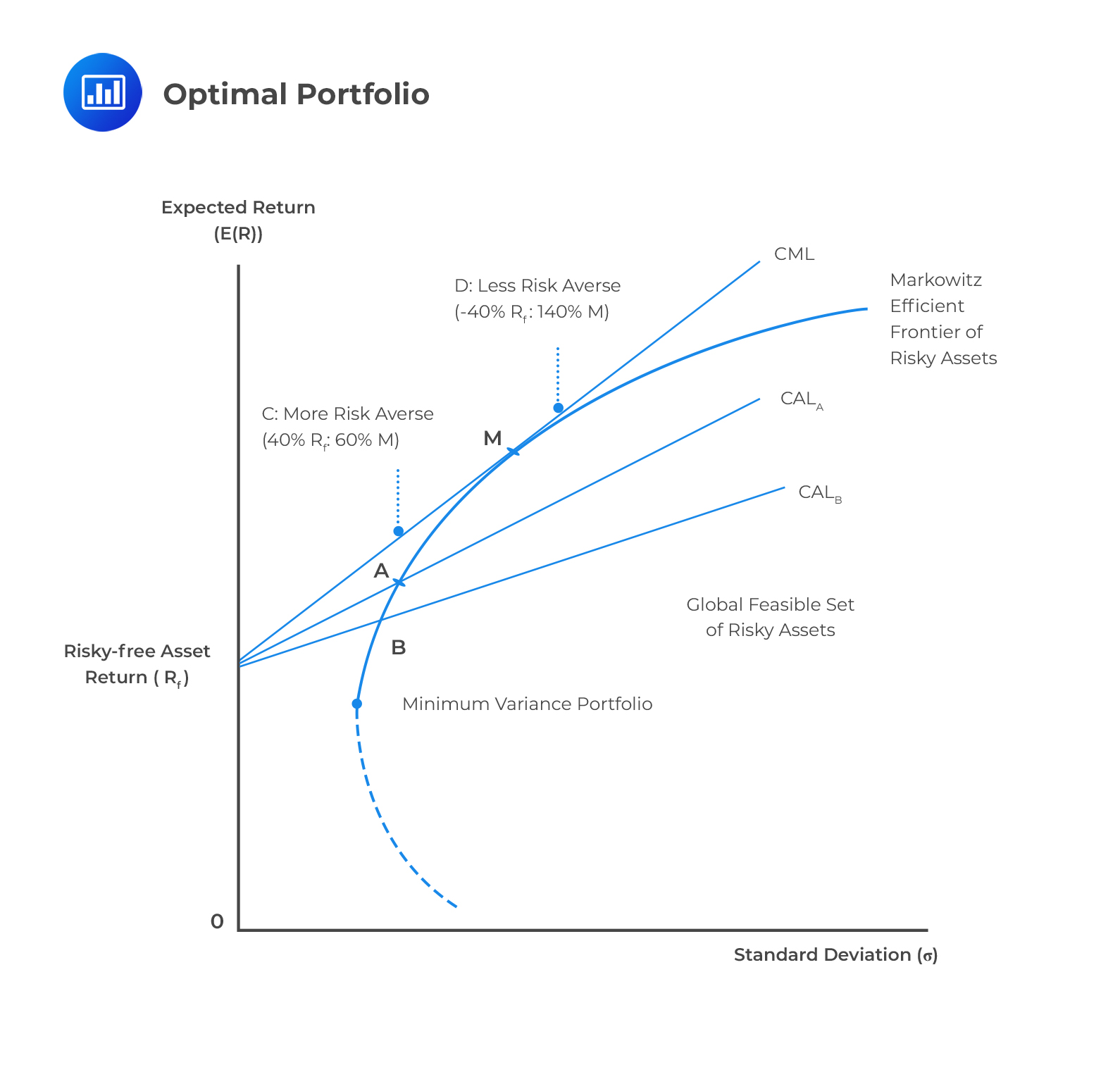
As the text notes, adding constraints can never improve the outcome of a minimization problem. Therefore, the variance of a constrained efficient portfolio will always be greater than or equal to the variance of its unconstrained counterpart with the same expected return. This means the new, constrained efficient frontier will lie to the right of the original one, as depicted in the image below.

This graph illustrates the unconstrained Markowitz Efficient Frontier (the blue curve). When no-short-selling is enforced, portfolios that required negative weights become infeasible. The new 'long-only' efficient frontier would be a segment of this curve, or a new curve entirely, that lies inside and to the right of this one, representing a less optimal set of choices.

3. Solving the Problem with Numerical Tools

Since we don't have a simple formula, we rely on numerical solvers to handle QP problems. These are standard tools in software like Excel, R, and Python. Your task is not to build the solver, but to correctly frame the portfolio problem in a way the solver can understand.

The process generally involves specifying:

Objective Function: The value you want to minimize or maximize (e.g., minimize portfolio variance x'Σx).
Changing Variables: The portfolio weights x that the solver can adjust.
Constraints: The rules the solution must follow (e.g., Σx_i = 1, x_i >= 0).

The following video provides an excellent, step-by-step tutorial on using Excel's built-in Solver to find an optimal portfolio, including how to add the crucial no-short-selling constraint.

Portfolio Optimization in Excel: Step by Step Tutorial

This video by Ryan O'Connell, CFA, FRM, provides a clear, practical walkthrough of using a numerical solver for portfolio optimization.

Focus on the section that demonstrates using the Excel Solver, from setting up the Solver. Observe how the objective (maximize Sharpe Ratio) is set, the variable cells (weights) are defined, and, most importantly, how the constraints are added. Notice the difference between a minimum weight of 0 (no short-selling) and a negative minimum weight (allowing short-selling).

This spreadsheet illustrates a typical setup for a portfolio optimization problem. The inputs are historical returns, from which expected returns and a covariance matrix are calculated. The solver's task is to find the optimal 'Portfolio %' weights that meet a specific goal, like minimizing risk for a target return, subject to constraints.

4. Finding Constrained Portfolios in Practice

Now let's apply this numerical approach to find the key portfolios we've discussed in previous lessons, but this time under the no-short-selling constraint. The Bookdown resource provides excellent examples using the R programming language, which, given your statistics background, should be quite accessible. The logic is identical to using the Excel Solver.

13 Portfolio Theory with Short Sales Constraints - Bookdown

This resource demonstrates how to frame the portfolio optimization problems for a quadratic programming solver in R.

Please read through the following sections to see how the theory is put into practice: Start with Section 13.4, "Quadratic Programming Problems", to understand how the portfolio problem is translated into the (D, d, A, b) matrices and vectors required by a typical QP solver. Work through Example 13.2 in Section 13.4.1. This shows how to find the Global Minimum Variance (GMV) portfolio with no short-selling. Notice that if the unconstrained GMV portfolio already has all positive weights, the constraint is "not binding" and the solution is the same. Next, study Example 13.3 in Section 13.4.2. This demonstrates finding an efficient portfolio for a target return and highlights how a binding constraint changes the portfolio's composition. Finally, read Section 13.4.3, "No short sales tangency portfolio". This is the most intricate part. It explains a clever method to find the constrained tangency (maximum Sharpe Ratio) portfolio by reformulating the problem, which is necessary because maximizing the Sharpe Ratio directly isn't a standard QP form.

The key takeaway is that for any given target return, the minimum variance achievable with a no-short-selling constraint will be equal to or higher than what's possible without the constraint. This difference in variance is the "cost" of the constraint.

Conclusion

Today we've bridged the gap between the idealized world of portfolio theory and the practical realities of investment management. By introducing constraints like no short-selling, the problem of finding an optimal portfolio shifts from an analytical exercise to a numerical one solved with quadratic programming.

Key Takeaways:

Real-world constraints, particularly the prohibition of short-selling ( $x_{i} \geq 0$ ), are common in portfolio management.
These constraints turn the mean-variance optimization into a Quadratic Programming (QP) problem.
Solving a constrained optimization requires numerical solvers (like Excel Solver or R's quadprog package) by defining an objective, variables, and constraints.
The constrained efficient frontier is never better than the unconstrained frontier; for a given expected return, a constrained portfolio will have an equal or higher level of risk.

You are now equipped to handle a wider and more realistic range of portfolio optimization problems. In our next module, we will shift our focus from constructing optimal portfolios to pricing the assets within them. We'll begin by exploring the Single-Index Model and then build towards the foundational Capital Asset Pricing Model (CAPM).