Tobin's Separation Theorem and Optimal Portfolios

Introduction

In our last lesson, we constructed the Capital Market Line (CML), which represents the most efficient set of portfolios available when you can combine risky assets with a risk-free asset. We saw that this optimal set is a straight line, a significant simplification from the curved efficient frontier of risky assets alone.

Today, we will formalize the profound implication of this discovery. This lesson focuses on the Tobin Separation Theorem, a cornerstone of modern portfolio theory. You will learn how this theorem splits the complex task of portfolio construction into two distinct, manageable steps. By the end of this lesson, you will be able to state the theorem and apply it to construct optimal portfolios for investors with different risk preferences, a key skill for your CM2 exam preparation.

1. The Separation Theorem: Two Decisions, Not One

The existence of the Capital Market Line leads to a powerful conclusion, first articulated by Nobel laureate James Tobin. The theorem states that the optimal investment strategy for any investor can be separated into two independent decisions:

The Investment Decision: This involves identifying a single optimal portfolio of risky assets. This portfolio is the same for every investor, regardless of their risk tolerance. It is the portfolio that offers the highest possible reward per unit of risk.
The Financing Decision: This involves deciding how to allocate one's capital between the risk-free asset and that single optimal risky portfolio. This decision is personal and depends entirely on the individual investor's unique risk aversion.

This is why it's called a "separation" or "two-fund" theorem. Every investor, from the most cautious to the most aggressive, should hold the same two "funds": the risk-free asset and the one optimal basket of risky securities. Their personal preferences only determine the mix between these two.

The document below provides a concise explanation of this idea.

[PDF] Chapter II. Mean-Variance Portfolio Choice

This excerpt from a chapter by Ronald Balvers explains the separation principle clearly.

Please read the section titled "An arbitrary number of risky assets plus a riskless asset". Focus on how all investment opportunities on the CML can be generated by combining just two portfolios: the tangency portfolio and the risk-free asset.

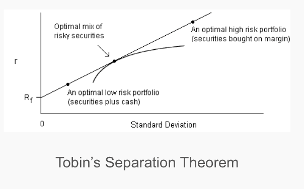
The image below, "Tobin's Separation Theorem," perfectly illustrates this concept.

This graph shows the efficient frontier of risky assets (the curve). The single "Optimal mix of risky securities" is the tangency portfolio. The straight line is the CML, representing all possible combinations of the risk-free asset (with return $R_f$) and this optimal risky portfolio. A risk-averse investor chooses a low-risk portfolio with securities plus cash, while a risk-tolerant investor borrows on margin to invest more heavily in the same optimal mix.

2. Decision 1: Identifying the Optimal Risky Portfolio

The first, and purely technical, task is to identify that single "optimal mix of risky securities." As we saw last lesson, this is the tangency portfolio—the point where the CML touches the efficient frontier. But how do we find it mathematically?

The key is to find the portfolio of risky assets that maximizes the Sharpe Ratio. The Sharpe Ratio, as you'll recall, is the slope of the Capital Allocation Line:

Sharpe Ratio = \frac{E [ R _{p} ] - R _{f}}{σ _{p}}

Where $E [R_{p}]$ and $σ_{p}$ are the expected return and standard deviation of the risky portfolio $p$ , and $R_{f}$ is the risk-free rate.

The following video provides a clear visual explanation of finding this tangency portfolio.

Efficient Frontier and Portfolio Optimization Explained | The Ultimate Guide

This video by Ryan O'Connell, CFA, FRM, gives a great conceptual overview of combining the risk-free rate with the efficient frontier to find the optimal portfolio.

Watch from the start of the segment to see how the line from the risk-free rate finds the point of tangency on the efficient frontier. Then continue watching from the next section where the Sharpe Ratio is defined and explained as the metric we are maximizing.

For a portfolio of N assets, this optimization problem can be solved using calculus and matrix algebra. Given your background in statistics, you might appreciate seeing the formal solution. The weights, $t$ , of the tangency portfolio are given by:

t = \frac{Σ ^{- 1} ( μ - R _{f} \cdot 1 )}{1 ^{'} Σ ^{- 1} ( μ - R _{f} \cdot 1 )}

Where:

$μ$ is the vector of expected returns of the risky assets.
$Σ$ is the covariance matrix of the risky assets.
$R_{f}$ is the risk-free rate.
$1$ is a vector of ones.

While the derivation is complex, the result is an objective formula. Given the same inputs for returns, risks, and correlations, every analyst will arrive at the same composition for the optimal risky portfolio.

3. Decision 2: The Financing Decision

Once the single optimal risky portfolio (let's call it $τ$ ) is identified, the second decision is purely personal. An investor must decide what proportion of their wealth, $x_{τ}$ , to invest in this portfolio, with the remaining proportion, $(1 - x_{τ})$ , invested in the risk-free asset.

Risk-averse investors will choose a small $x_{τ}$ (e.g., $0 < x_{τ} < 1$ ), effectively lending part of their wealth at the risk-free rate. Their portfolio lies on the CML between the risk-free asset and the tangency portfolio.
Risk-tolerant investors might choose $x_{τ} > 1$ . This means they borrow money at the risk-free rate and invest their entire capital, plus the borrowed funds, into the tangency portfolio. Their portfolio lies on the CML beyond the tangency point.

The formulas for the expected return ( $μ_{p}^{e}$ ) and standard deviation ( $σ_{p}^{e}$ ) of the final, efficient portfolio are straightforward linear combinations:

μ_{p}^{e} = R_{f} + x_{τ} (μ_{τ} - R_{f})

σ_{p}^{e} = x_{τ} σ_{τ}

Where $μ_{τ}$ and $σ_{τ}$ are the expected return and standard deviation of the tangency portfolio.

The following resource provides excellent numerical examples of this second step, showing how to calculate the required allocation $x_{τ}$ to achieve a target return or a target level of risk.

Econ 424/CFRM 462 Portfolio Theory with Matrix Algebra

This document by Eric Zivot formally states the "Mutual Fund Separation Theorem" and provides clear, practical examples.

Please read the section "Mutual Fund Separation Theorem". Then, carefully work through the two examples that follow, where the goal is to find a portfolio for a target risk and a target expected return. This directly addresses the "apply" part of today's learning outcome.

4. A Complete Practical Walkthrough

To bring everything together, let's walk through the entire process numerically. The following video demonstrates in Excel how to start with raw asset data and perform both steps of the Tobin separation process. This hands-on approach is invaluable for cementing your understanding for the exam.

Graph The Efficient Frontier And Capital Allocation Line In Excel

This Excel tutorial by Ryan O'Connell, CFA, FRM, is a perfect practical application of the concepts we've discussed.

Follow along with the video's steps: Data Preparation (this segment): Observe how daily returns, average returns (expected returns), standard deviations, and covariance are calculated from price data. The Investment Decision (this segment): See how the Sharpe Ratio is calculated for many different portfolios and how the optimal portfolio is identified as the one with the maximum Sharpe Ratio. This is Decision 1 in action. The Financing Decision (this segment): Watch as the efficient frontier is plotted and the CML is constructed by combining the optimal portfolio with the risk-free asset. This demonstrates how investors can achieve any point on the CML by lending or borrowing (Decision 2).

Conclusion

This lesson has formalized a critical insight from our work on the Capital Market Line. The Tobin Separation Theorem shows that the portfolio construction process can be elegantly split into two parts. The first is an objective, technical exercise to find the single best portfolio of risky assets, which is identical for everyone. The second is a subjective choice about how to blend this risky portfolio with a risk-free asset to match one's personal comfort with risk.

Key Takeaways:

Tobin's Separation Theorem: The investment decision is separated into two funds: the optimal risky (tangency) portfolio and the risk-free asset.
Investment Decision: Find the one tangency portfolio that maximizes the Sharpe Ratio. This task is objective and the same for all investors.
Financing Decision: Choose a personal allocation between the tangency portfolio and the risk-free asset (lending or borrowing) to match your individual risk aversion.

This powerful idea has practical implications, supporting the strategy of investing in a broad market index fund (as a proxy for the tangency portfolio) and adjusting overall risk with cash or leverage.

In our next lesson, we will build on this foundation by exploring how to solve these portfolio optimization problems when we introduce real-world constraints, such as a prohibition on short-selling.

Recommended resources