One-Period Binomial Tree: Risk-Neutral Probability

Introduction

In our last lesson, we identified the six key factors that influence an option's price, giving us a qualitative understanding of how value changes. We now move from the "what" to the "how," by starting to build a quantitative model for pricing options. This lesson marks our first step into the practical mechanics of derivative valuation, a core skill for the CM2 exam.

We will introduce the one-period binomial model, a simple yet powerful framework that assumes an asset's price can only move to one of two possible states over a single time step. Within this model, we will define and calculate a crucial concept: risk-neutral probability. Your background in probability theory will be particularly useful here, as we'll explore how this special, constructed probability allows us to price complex securities in a surprisingly straightforward manner, without needing to forecast the real-world likelihood of market movements.

The One-Period Binomial Framework

Imagine we want to price an option that expires in the near future. The binomial model simplifies the infinite possibilities of stock price movements into a manageable, discrete structure. In a single period, we assume the current stock price, $S_{0}$ , can only do one of two things:

Move up to a new price $S_{1}^{u}$ .
Move down to a new price $S_{1}^{d}$ .

These movements are defined by an up-factor ( $u$ ) and a down-factor ( $d$ ), where $u > 1$ and $d < 1$ . The future prices are simply:

S_{1}^{u} = S_{0} \times u

S_{1}^{d} = S_{0} \times d

Often, to prevent arbitrage within the model itself, these factors are set as reciprocals, such that $d = 1/ u$ .

The following video provides a clear, quick introduction to this setup.

Binomial Option Pricing Model (Calculations for CFA® and FRM® Exams)

This video, "Binomial Option Pricing Model" from AnalystPrep, is focused on the practical calculations required for CFA and FRM exams, which aligns perfectly with our goal.

Watch the following segments to familiarize yourself with the binomial tree structure: Basic Idea: Watch this part for the core assumption of two states. The video mentions multi-period trees, but for now, we're focused only on the first step from S_0 to S_u and S_d. Building the Stock Tree: This segment shows how to apply the up and down factors to a starting price to find the two possible future stock prices.

Why Real-World Probabilities Don't Work

Now that we have a model for stock prices, how do we price an option? A natural first thought, especially for a statistician, would be to:

Estimate the real-world probabilities ( $p$ ) of the stock going up and ( $1 - p$ ) of it going down.
Calculate the option's payoff in each state.
Compute the expected payoff: $p \times Payoff(up) + (1 - p) \times Payoff(down)$ .
Discount this expected payoff back to today at an appropriate risk-adjusted rate.

This seems logical, but it contains two major problems: What are the correct probabilities, and what is the correct discount rate? In finance, we sidestep this entire issue through the principle of no-arbitrage. Instead of guessing at probabilities and risk, we find the price by constructing a perfect hedge.

The following video masterfully explains why the real-world probability approach is flawed and introduces the far more robust concept of pricing by replication.

Binomial Options Pricing Model Explained

The video "Binomial Options Pricing Model Explained" by Perfiliev Financial Training provides exceptional intuition on the theory behind risk-neutral pricing.

Please watch these crucial segments: The Flawed Approach: Watch this section to understand why using real-world probabilities leaves an option seller exposed to unhedged risk. The Hedging Solution: This key segment shows how to create a risk-free portfolio by combining the option with a specific number of shares of the underlying stock (a technique called delta-hedging). The value of this portfolio is the same whether the stock goes up or down. Probabilities Don't Matter: This part explicitly concludes that because the price is determined by this hedge, the actual real-life probabilities of the stock's movement have no impact on the option's fair value.

The key takeaway is this: we can form a portfolio of the underlying stock and a risk-free bond that exactly replicates the option's payoffs. Because this replicating portfolio has the same future value as the option in all possible states, it must have the same price today. If it didn't, an arbitrage opportunity would exist.

The Shortcut: Risk-Neutral Probability

Calculating the composition of the replicating portfolio (finding the delta and bond amount) for every option price can be cumbersome. Fortunately, the math of replication can be rearranged into an elegant and intuitive formula that looks like a discounted expected value. This is where risk-neutral probability comes in.

It is a constructed probability measure (let's call it $π$ ) that, if it were the true probability, would make the expected return on the stock equal to the risk-free rate. By using $π$ to calculate the expected option payoff and then discounting at the risk-free rate, we arrive at the exact same price as the one derived from the more complex replication argument.

This allows us to pretend we live in a "risk-neutral world" for the purpose of calculation. In this world:

All investors are indifferent to risk.
The expected return on all assets is the risk-free rate.

The formula for the risk-neutral probability of an up-move is derived directly from these conditions.

Risk-Neutrality in Derivative Pricing | CFA Level 1

This article from AnalystPrep provides the precise formulas we need.

Please read the first part of the article, focusing on the two key formulas. Start from the beginning and read down to the definition. Pay close attention to the formula for \pi (risk-neutral probability) and the formula for c_0 (the call price), which uses \pi. The article uses R^u and R^d for the up and down gross returns, which are the same as our u and d factors.

The crucial formula for the risk-neutral probability of an up move, using discrete compounding, is:

π = \frac{( 1 + r ) - d}{u - d}

Where:

$r$ is the risk-free rate for the period.
$d$ is the down-factor.
$u$ is the up-factor.

The risk-neutral probability of a down move is simply $1 - π$ .

Worked Example

Let's put this into practice and solidify the calculation. We will use the example from the AnalystPrep article you just reviewed.

Problem: A one-year call option is being considered on a stock.

Current stock price ( $S_{0}$ ): $80
Exercise price ( $K$ ): $85
Risk-free rate ( $r$ ): 4% per year
The stock price is expected to go up or down by 30% over the year.

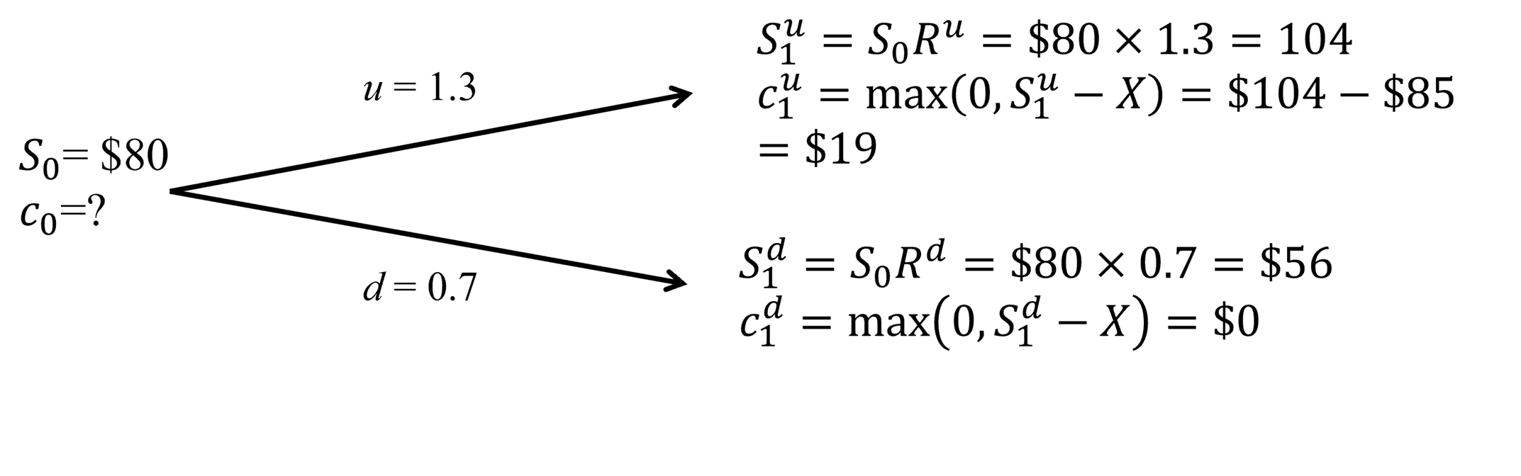
Step 1: Construct the Binomial Tree

First, we define the parameters and map out the possible future states for the stock and the option.

Up-factor $u = 1 + 0.30 = 1.3$
Down-factor $d = 1 - 0.30 = 0.7$
Up-state stock price $S_{1}^{u} = $80 \times 1.3 = $104$
Down-state stock price $S_{1}^{d} = $80 \times 0.7 = $56$

Next, we calculate the option's payoff (its intrinsic value) at expiration in each state.

Payoff in up-state $c_{1}^{u} = max (0, S_{1}^{u} - K) = max (0, $104 - $85) = $19$
Payoff in down-state $c_{1}^{d} = max (0, S_{1}^{d} - K) = max (0, $56 - $85) = $0$

This entire setup is visualized in the following diagram.

This diagram shows the one-period binomial tree for the stock price (S) and the corresponding call option payoffs (c). The initial stock price is \$80, and it can move up to \$104 or down to \$56. The call option payoffs are \$19 in the up-state and \$0 in the down-state.

Step 2: Calculate the Risk-Neutral Probability ( $π$ )

This is the main goal of our lesson. We plug the values for the risk-free rate, up-factor, and down-factor into our formula:

π = \frac{( 1 + r ) - d}{u - d} = \frac{( 1 + 0.04 ) - 0.7}{1.3 - 0.7} = \frac{1.04 - 0.7}{0.6} = \frac{0.34}{0.6} \approx 0.5667

So, the risk-neutral probability of the stock price increasing to $104 is approximately 56.67%. The probability of it decreasing is $1 - 0.5667 = 0.4333$ , or 43.33%.

Note that this calculated probability has nothing to do with any real-world forecast of the stock's direction; it is purely a function of the model's parameters ( $u, d$ ) and the risk-free rate ( $r$ ).

The AnalystPrep article walks through this exact calculation.

Risk-Neutrality in Derivative Pricing | CFA Level 1

This section applies the formula we just learned to the problem we are solving.

Review the section titled the example. Follow the calculation of the risk-neutral probability of an upward move, \pi, which is the primary objective of this lesson.

Conclusion

In this lesson, we established the foundational model for discrete-time option pricing. We moved beyond qualitative factors and began building a quantitative framework. You now know how to construct a simple world with two future states and, most importantly, how to calculate the risk-neutral probability that is the key to pricing any derivative within it.

Key Takeaways:

The one-period binomial model simplifies future asset price movements into two discrete states: an up-move and a down-move.
Pricing derivatives using real-world probabilities is problematic because it requires subjective forecasts and determining a risk-adjusted discount rate.
The no-arbitrage principle allows us to price an option by creating a replicating portfolio of the underlying and a risk-free bond, which eliminates risk and uncertainty.
Risk-neutral probability ( $π$ ) is a mathematical construct that provides a powerful shortcut to the replication method. It allows us to price options by calculating a discounted expected payoff, where the expectation is taken under $π$ and the discount rate is the risk-free rate.
The formula $π = ((1 + r) - d) / (u - d)$ is fundamental for finding this probability.

We have successfully calculated the risk-neutral probability. In our next lesson, we will use this result to complete the pricing process. We will extend the one-period model to a multi-period binomial tree, allowing us to value options with longer times to expiration and see how the price evolves through time.