Utility Functions: Non-Satiation & Risk Aversion

1. From Preferences to Utility Functions

At its core, economics is about choices. To model choice, we first need a way to describe preferences. We can do this by making a few simple, yet powerful, assumptions about how people rank different outcomes.

Professor Jonathan Gruber from MIT provides a very clear explanation of the three foundational assumptions that allow us to translate subjective preferences into a mathematical utility function.

If a person's preferences satisfy these three conditions, we can represent them with a utility function, denoted as $U(W)$. This function assigns a numerical score (utility) to a certain level of wealth, $W$, in a way that reflects the person's preferences. If you prefer outcome A to outcome B, then the utility of A must be higher than the utility of B: $U(A)>U(B)$.

It is crucial to understand that these utility numbers are ordinal, not cardinal. This means they only serve to rank the choices. A utility score of 200 is better than 100, but it doesn't mean it's "twice as good." The numbers themselves don't have an intrinsic meaning beyond establishing a pecking order for your preferences.

2. The Shape of a Utility Function: Non-satiation and Risk Aversion

The shape of an individual's utility function tells us about their personality as an investor. We can describe this shape using its first and second derivatives.

Non-satiation: "More is Better"

The assumption of non-satiation means that utility should always increase as wealth increases. An investor will always prefer having more money to having less. Mathematically, this means the utility function must be an increasing function of wealth.

This implies that its first derivative, the slope of the utility curve, must be positive. This slope is called the marginal utility of wealth.

• Condition for Non-satiation: $U^{\prime }(W)=\frac{dU}{dW}>0$

A positive marginal utility simply means that for every extra dollar you get, your total satisfaction, or utility, goes up.

Risk Aversion: Diminishing Marginal Utility

Now for the more interesting part. How does utility change as you get wealthier? Consider this: gaining an extra $1,000 means a lot more to someone with a net worth of $5,000 than it does to someone with a net worth of $5 million. While both individuals' utility increases (non-satiation), the amount by which it increases is smaller for the wealthier person. This idea is called diminishing marginal utility.

This concept is the cornerstone of risk aversion. Because the utility gained from an extra dollar is less than the utility lost from the preceding dollar, a person with diminishing marginal utility will reject a fair bet. For example, a 50/50 gamble to win or lose $1,000 has an expected value of $0, but it is unattractive. The potential pain (utility lost) from losing $1,000 outweighs the potential pleasure (utility gained) from winning $1,000.

Mathematically, diminishing marginal utility means the slope of the utility function gets flatter as wealth increases. In other words, the first derivative, $U^{\prime }(W)$, is a decreasing function. This implies that the second derivative must be negative. A function with a positive first derivative and a negative second derivative is concave.

• Condition for Risk Aversion: $U^{\prime \prime }(W)=\frac{d^{2}U}{d{W}^2}<0$

Therefore, a risk-averse investor is defined as one who has a concave utility function.

3. Visualizing Risk Preferences

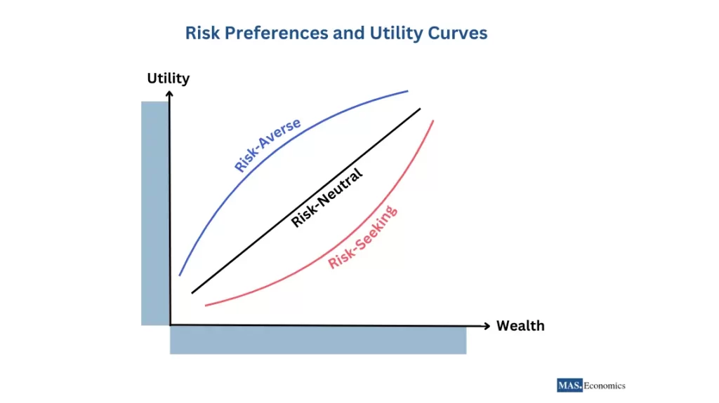
We can classify investors into three main categories based on their attitude towards risk, which is directly reflected in the shape of their utility function.

1. Risk-Averse: Prefers a certain outcome over a gamble with the same expected value. Their utility function is concave ($U^{\prime \prime }(W)<0$), reflecting diminishing marginal utility. Most traditional financial models assume investors are risk-averse.

2. Risk-Neutral: Is indifferent between a certain outcome and a gamble with the same expected value. They only care about the expected return, not the risk. Their utility function is a straight line ($U^{\prime \prime }(W)=0$), reflecting constant marginal utility.

3. Risk-Seeking (or Risk-Loving): Prefers a gamble over a certain outcome with the same expected value. They get an extra thrill from the uncertainty itself. Their utility function is convex ($U^{\prime \prime }(W)>0$), reflecting increasing marginal utility. This might describe someone who enjoys playing the lottery, where the expected value is typically negative.

The following video provides an excellent summary of these three types and illustrates their choices with a simple gambling example.

4. Common Utility Functions in Finance

To apply these concepts, economists and actuaries use several standard utility functions. Let's briefly look at a few common examples and check their properties. This will set the stage for our next lesson, where we'll use these functions for calculations.

For each function below, we can verify the conditions for non-satiation ($U^{\prime }(W)>0$) and risk aversion ($U^{\prime \prime }(W)<0$).

• Logarithmic Utility: $U(W)=\ln (W)$

  • $U^{\prime }(W)=1/W$. For positive wealth $W$, this is positive. (Satisfies non-satiation)
  • $U^{\prime \prime }(W)=-1/W^2$. This is always negative. (Satisfies risk aversion)

• Power Utility: $U(W)=\frac{W^{1-\gamma }}{1-\gamma }$ (where $\gamma >0,\gamma \ne 1$)

  • $U^{\prime }(W)=W^{-\gamma }$. For positive wealth $W$, this is positive. (Satisfies non-satiation)
  • $U^{\prime \prime }(W)=-\gamma W^{-\gamma -1}$. Since $\gamma >0$, this is always negative. (Satisfies risk aversion)
  • Note: The logarithmic utility function is a special case of the power utility function as $\gamma$ approaches 1.

• Exponential Utility: $U(W)=-e^{-aW}$ (where $a>0$)

  • $U^{\prime }(W)=a{e}^{-aW}$. Since $a>0$, this is always positive. (Satisfies non-satiation)
  • $U^{\prime \prime }(W)=-a^2{e}^{-aW}$. This is always negative. (Satisfies risk aversion)

This is just a preview. For a more formal list, you can refer to the following resource.

Conclusion

In this lesson, we laid the mathematical foundation for modeling rational choice under uncertainty. We have moved from the intuitive idea of preferences to the formal structure of a utility function.

Here are the key takeaways:

• A utility function $U(W)$ numerically represents an individual's preferences, assuming those preferences are complete, transitive, and non-satiated.
• Non-satiation ("more is better") implies that the utility function is increasing, meaning its first derivative is positive: $U^{\prime }(W)>0$.
• Risk aversion is characterized by diminishing marginal utility. This means the utility function is concave, and its second derivative is negative: $U^{\prime \prime }(W)<0$.
• The shape of the utility function defines the investor type: concave for risk-averse, linear for risk-neutral, and convex for risk-seeking.

We have now defined what a utility function is and what its shape tells us. In our next lesson, we will put this tool to work. We will learn how to use the Expected Utility Theorem to rank different risky investment opportunities and make optimal choices. We'll also calculate the certainty equivalent—the guaranteed amount of money that would make you just as happy as taking a gamble.