Lorentz Force and Magnetic Pressure in Coil Windings

1. The Lorentz Force and Magnetic Pressure

The fundamental source of force on any current-carrying wire in a magnetic field is the Lorentz force. For a small segment of wire $d\vec{l}$ carrying current $I$, the force $d\vec{F}$ is:

$d\vec{F}=I(d\vec{l}\times \vec{B})$

It is often more convenient to work with a continuous current density $\vec{j}$ (in A/m²) and the corresponding force density $\vec{f}$ (in N/m³):

$\vec{f}=\vec{j}\times \vec{B}$

This is a body force, meaning it acts throughout the entire volume of the conductor. To find the total force on a component, we must integrate this density over its volume.

A very useful and intuitive concept for understanding the overall effect of these forces is magnetic pressure. The magnetic field stores energy, and this energy density acts like a pressure pushing on the conductors that create it.

To build a strong intuition for this concept, let's watch a classic lecture segment from Prof. Walter Lewin.

As Prof. Lewin demonstrates, the magnetic pressure $p_m$ is given by:

$p_m=\frac{B^2}{2{\mu }_0}$

This simple formula is incredibly powerful. For a 40 T field, typical of a high-end resistive magnet, the magnetic pressure is $p_m=(40^2)/(2\cdot 4\pi \times 10^{-7})\approx 637\times 10^6$ Pa, or about 637 MPa. This is comparable to the yield strength of many high-strength steels, giving you an immediate sense of the immense forces that need to be managed.

The following document provides a concise summary of these foundational concepts.

2. Deconstructing the Force: Radial and Axial Components

The magnetic pressure gives us a sense of the overall magnitude, but to design a robust magnet, we need to know the direction of the forces. Let's analyze the force density vector $\vec{f}=\vec{j}\times \vec{B}$ for a standard solenoid.

1. Current Density $\vec{j}$: In a simple solenoid, the wire is wound in hoops, so the current flows in the azimuthal direction: $\vec{j}=j_{\theta }\hat{\theta }$.
2. Magnetic Field $\vec{B}$: As we learned in the last lesson, the field inside the winding has two main components: a strong axial field $B_z$ and a weaker radial field $B_r$ that peaks at the coil ends: $\vec{B}=B_z\hat{z}+B_r\hat{r}$.

Now, let's compute the cross product:
$\vec{f}=j_{\theta }\hat{\theta }\times (B_z\hat{z}+B_r\hat{r})=j_{\theta }{B}_z(\hat{\theta }\times \hat{z})+j_{\theta }{B}_r(\hat{\theta }\times \hat{r})$
Using the relations for cylindrical unit vectors ($\hat{\theta }\times \hat{z}=\hat{r}$ and $\hat{\theta }\times \hat{r}=-\hat{z}$), we get:

$\vec{f}=\underset{f_r}{\underbrace{(j_{\theta }{B}_z)}}\hat{r}\underset{f_z}{\underbrace{-(j_{\theta }{B}_r)}}\hat{z}$

This result is profoundly important. It tells us the force has two distinct components:

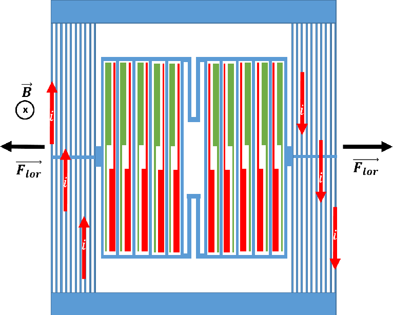
• Radial Force ($f_r$): The product of the azimuthal current and the strong axial field creates a purely outward radial force. This is often called hoop force, and it tries to burst the magnet open. This is the force responsible for the hoop stress we will study later.

• Axial Force ($f_z$): The product of the azimuthal current and the radial field creates an axial force. Since $B_r$ has opposite signs on either side of the magnet's midplane (it points outward at the ends), this force is directed inward, compressing the coil towards its center.

3. Calculating the Force Distribution

To calculate the precise force at every point in the winding, we must combine the field calculation methods from the last lesson with the Lorentz force law. The filamentary model you were introduced to is perfectly suited for this. The computational procedure is as follows:

1. Discretize: The coil is modeled as a collection of N straight wire "filaments."
2. Calculate Field: For each filament i, calculate the magnetic field ${\vec{B}}_i$ at its center, which is the vector sum of the fields produced by all other filaments ($j\ne i$).
   ${\vec{B}}_i={\sum }_{j\ne i}{\vec{B}}_j(\text{at center of }i)$
3. Calculate Force: With the current $I$ and vector length $d{\vec{l}}_i$ of the filament known, the force on that segment is calculated directly.
   ${\vec{F}}_i=I(d{\vec{l}}_i\times {\vec{B}}_i)$

By repeating this for every filament, we can map the entire force distribution vector field throughout the coil.

The dissertation by Szabolcs Rembeczki, which we used in the last lesson, implements this exact method. Let's examine how it is described and what the results look like.

From analyzing these plots, several key features of force distribution in a conventional solenoid become apparent:

• The radial force is large, positive (outward), and relatively constant along the central portion of the coil. It is the dominant force component.
• The axial force is negligible at the center ($x=0$) and grows to its maximum value at the ends, pointing inwards.
• The azimuthal force is negligible in a standard solenoid. (The large azimuthal forces seen in the "force-reduced" examples are a consequence of their special helical winding geometry, designed to trade radial force for azimuthal force).

Conclusion

In this lesson, we have connected the magnetic field profile of a coil directly to the mechanical forces it must endure. These forces are not just a theoretical curiosity; they are a tangible, destructive reality that every high-field magnet designer must confront.

Key Takeaways:

• The fundamental force is the Lorentz force, expressed as a density $\vec{f}=\vec{j}\times \vec{B}$.
• The concept of magnetic pressure, $p_m=B^2/(2{\mu }_0)$, provides a powerful estimate for the scale of the forces involved.
• In a standard solenoid, the force vector can be decomposed into two main components:
  • A radial (hoop) force ($\propto j_{\theta }{B}_z$) that tries to burst the coil.
  • An axial force ($\propto j_{\theta }{B}_r$) that compresses the coil towards its midplane.
• Numerical methods, such as the filamentary model, are essential for calculating the detailed force distribution in complex coil geometries, allowing designers to map the force vectors throughout the windings.

Next Lesson Preview:
We have now calculated the forces. The next logical question is: what effect do these forces have on the materials of the coil? In the next lesson, we will begin our exploration of solid mechanics by defining stress, strain, and elastic modulus, and applying Hooke's law. This will allow us to translate the force distribution we calculated today into the internal stresses and physical deformations that the magnet components experience, which is the heart of mechanical design.