Coil Magnetic Field Analysis

Hello! Welcome to your next lesson in our course on high-field magnet design.

In our last lesson, we established the foundational design equation for a simple solenoid, linking its central field $B_{0}$ to its geometry ( $α, β$ ) and the current density $j$ . We saw how to make a first-order estimate for the dimensions of a coil required to produce a target field.

However, the field is only perfectly uniform and axial at the exact geometric center. For any real experiment, we need to know how the field behaves away from this point. This brings us to today's learning outcome: Calculate the axial and radial magnetic field profiles for a designed coil and assess the field homogeneity in the sample region.

We will move beyond the single value $B_{0}$ to determine the full magnetic field vector $B (r, z) = B_{z} (r, z) z^+ B_{r} (r, z) r^$ at any point. This is crucial for two reasons:

Assessing Field Quality: Experiments rely on a known and uniform magnetic field. We need to quantify the volume over which the field is sufficiently homogeneous for a given measurement.
Calculating Mechanical Forces: The immense Lorentz forces that threaten to destroy a pulsed magnet depend on the magnetic field at the location of the current-carrying wires. Understanding the field profile within the windings is the first step toward calculating these forces, which is the topic of our next lesson.

Let's begin by looking at the object we are modeling.

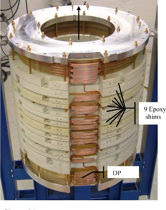
Cutaway View of a Multi-Turn Pulsed Magnet Coil — This image shows the internal structure of a multi-layer pulsed magnet, with its copper windings and insulation. Our goal is to calculate the magnetic field everywhere within the bore and throughout the windings of such a structure.

1. The On-Axis Field Profile: $B_{z} (0, z)$

In the previous lesson, we focused only on the field at the center, $z = 0$ . The formula for the on-axis field of a thin solenoid of radius $R$ and length $L$ at an arbitrary axial position $z$ (measured from the center) is:

$B_{z} (0, z) = \frac{μ _{0} n I}{2} [\frac{L /2 - z}{R ^{2} + ( L /2 - z ) ^{2}} + \frac{L /2 + z}{R ^{2} + ( L /2 + z ) ^{2}}]$

Here, $n I$ is the current per unit length. For a thick solenoid, we integrate this expression over the radius from $a_{1}$ to $a_{2}$ . The result is a more complex version of the Fabry formula we saw last time. While the full derivation is cumbersome, the key result is a field that is maximum at the center ( $z = 0$ ) and falls off as we approach the ends of the coil.

You can see a plot of this on-axis field profile in the resource below, which we will be using throughout this lesson.

Design and Optimization of Force-Reduced High Field ...

The following dissertation by Szabolcs Rembeczki presents a comprehensive design study of high-field solenoids. We will first look at its simulation of the on-axis field.

Please find Section 4.2.1, 'Magnetic Field in the Bore', and examine Figure 4.5. This figure shows the calculated on-axis axial field profile (B_{ax}) for several solenoids of the same length but different wire pitch angles. Notice how the field is relatively flat near the center (x=0) and then drops off towards the ends of the coil (indicated by magenta lines).

2. Off-Axis Fields: The Full $B (r, z)$ Profile

Calculating the field at an off-axis point ( $r > 0$ ) is significantly more complex. The radial symmetry is broken, and a radial field component, $B_{r}$ , appears. A direct integration of the Biot-Savart law leads to expressions involving elliptic integrals.

Given your mathematical background, you will find the following derivation from a classic NASA technical note illuminating. It lays out the problem clearly, starting from the magnetic vector potential.

NOTE

The NASA technical note 'THE MAGNETIC FIELD OF A FINITE SOLENOID' by Callaghan and Maslen provides a complete analytical solution for the field of a thin solenoid in terms of elliptic integrals. This is a foundational piece of work for magnet design.

Please read the 'INTRODUCTION' and 'DERIVATION OF EQUATIONS' sections (pages 1-5). Follow the derivation from the vector potential A_\theta (eq. 3) to the expressions for the radial field B_r (eq. 9) and axial field B_z (eq. 11). Pay attention to how these final forms depend on the complete elliptic integrals K(k) and E(k), and the Heuman lambda function \Lambda_0(\beta, k), which are functions of the geometry.

The key takeaways from this derivation are:

The field components $B_{z} (r, z)$ and $B_{r} (r, z)$ for a thin solenoid can be expressed analytically.
For a thick solenoid, one would need to integrate these complex expressions over the radius ( $a_{1}$ to $a_{2}$ ). This is almost always done numerically in modern design codes.
From Maxwell's equations ( $\nabla \cdot B = 0$ ), we know that if the axial field $B_{z}$ changes with $z$ , there must be a non-zero radial field $B_{r}$ . Specifically, in cylindrical coordinates: $\frac{1}{r} \frac{\partial ( r B _{r} )}{\partial r} = - \frac{\partial B _{z}}{\partial z}$ . This is why $B_{r}$ is largest near the ends of the coil, where $B_{z}$ changes most rapidly.

3. Field Homogeneity in the Sample Region

The NASA note's plots of the dimensionless field components are extremely useful for understanding field homogeneity. A magnet's "good field" region is the volume where the field deviates from the central value by less than a specified tolerance (e.g., 1%, 0.1%, or even smaller for applications like NMR).

NOTE

Now, let's analyze the graphical results of the derivation to understand field homogeneity.

Please read the 'Discussion' section (page 6) and examine the plots in Figure 1 (axial field) and Figure 2 (radial field). These plots show the field distribution for solenoids with different length-to-radius ratios (L/a). Focus on how the shape of the coil affects the field uniformity. Note how for longer solenoids (larger L/a), the lines of constant field become flatter and more widely spaced near the center, indicating a more homogeneous field.

As the note explains, and the figures clearly show:

Longer solenoids produce more homogeneous fields. For a very long coil ( $L / a \to \infty$ ), the field becomes perfectly uniform inside.
The radial field $B_{r}$ is zero on the axis ( $r = 0$ ) and increases as you move outward. It is the primary contributor to field inhomogeneity near the magnet's midplane.
The axial field $B_{z}$ decreases as you move radially outward and axially away from the center.

Test your understanding!

Imagine you are designing a magnet for an experiment that requires a field homogeneity of about 1% over a sample region that occupies the central 50% of the bore radius ( $r / a \leq 0.5$ ) and central 20% of the coil length ( $2 z / L \leq 0.2$ ).

Looking at the plots in Figure 1 of the NASA note, which coil would be a better choice: one with $L / a = 4$ or one with $L / a = 10$ ? Why?

Show answer

The coil with $L / a = 10$ would be a much better choice.

Let's look at the plots for the axial field $B_{z}$ .

For $L / a = 4$ (Figure 1(d)), the field at the center is $\frac{4 π B _{z}}{μ _{0} n I} \approx 3.8$ . At the edge of our sample region ( $r / a = 0.5, 2 z / L = 0.2$ ), the field value contour is roughly 3.6. This is a drop of $(3.8 - 3.6) /3.8 \approx 5%$ , which is too inhomogeneous.
For $L / a = 10$ (Figure 1(f)), the central field value is nearly 4.0. Within our entire sample region ( $r / a \leq 0.5, 2 z / L \leq 0.2$ ), the field lines are very flat and all lie well above the 3.9 contour. The deviation from the central value is clearly much less than 1%.

This illustrates the fundamental trade-off: achieving high homogeneity requires long coils, which are larger, more expensive, and may have other undesirable properties.

4. Field Profiles at the Windings

So far, we have focused on the field in the bore. Now, we shift our attention to the field within the conductor windings. This is essential for calculating the Lorentz forces in our next lesson.

The Rembeczki dissertation provides an excellent analysis of the field components calculated at the windings of a realistic multi-layer magnet design.

Design and Optimization of Force-Reduced High Field ...

Let's return to the Rembeczki thesis and examine the calculated field profiles at the winding locations for the conceptual 25 T magnet.

Please read Section 5.2, 'Magnetic Field Analysis', focusing on sub-section 5.2.2, 'Magnetic Field at the Winding' (pages 89-90). Study Figures 5.6, 5.7, and 5.8, which show the radial, axial, and azimuthal field components along the length of each of the three layers of the coil.

From this reading, you should note three critical behaviors:

Axial Field ( $B_{a x}$ ): As seen in Figure 5.7, the axial field is strong throughout the windings. It is highest on the innermost layer and decreases progressively for the outer layers. This strong axial field, crossing with the azimuthal current, will produce the main radial (hoop) force.
Radial Field ( $B_{r a d}$ ): Figure 5.6 shows that the radial field is very small in the central part of the coil but grows to large positive and negative peaks at the ends. This is the "end effect" we discussed earlier. This strong radial field at the ends, crossing with the azimuthal current, produces the powerful axial forces that try to stretch the coil or compress it towards the midplane.
Azimuthal Field ( $B_{a z}$ ): Figure 5.8 shows a significant azimuthal field. This is a special feature of the "force-reduced" coil design in the thesis, where the wires are wound at a pitch angle. In a standard solenoid with purely azimuthal currents, this component would be zero. This field interacts with the axial component of the current to modify the forces.

5. A Note on Calculation Methods

The analytical formulas involving elliptic integrals are invaluable for understanding the physics and for benchmarking. However, for a complex, multi-layer coil with varying current densities, designers rely on numerical methods.

The Rembeczki thesis uses a filamentary approximation. The idea is simple yet powerful:

The continuous winding is broken down into a large number of small, straight wire segments ("filaments").
The simple Biot-Savart law is used to calculate the field contribution from each individual filament at any point in space.
The total field is the vector sum of the contributions from all filaments.

This method is highly suited to your programming skills and is the basis for many specialized magnet design codes, including the PMDS software you're interested in. It's effectively a numerical integration of the Biot-Savart law. The accuracy of this method is confirmed in Appendix C of the thesis, where it's shown to agree well with commercial Finite Element Method (FEM) software.

Conclusion

In this lesson, we have moved from a single value for the central field to a comprehensive understanding of the entire magnetic field profile of a solenoid.

Key Takeaways:

The off-axis magnetic field of a solenoid has both axial ( $B_{z}$ ) and radial ( $B_{r}$ ) components, which can be calculated analytically for simple geometries using elliptic integrals.
Field homogeneity is a critical design parameter, determined primarily by the coil's aspect ratio ( $L / a$ ). Longer coils provide better homogeneity.
The field profile at the windings is different from the profile in the bore. In particular, the radial field component ( $B_{r}$ ) peaks at the ends of the coil.
Modern magnet design relies on numerical methods like the filamentary approximation or FEM to accurately compute field profiles in complex, real-world coil geometries.

Next Lesson Preview:
We now have the tools to calculate the $B$ field at any point in our coil. In the next lesson, we will use this knowledge to tackle one of the most critical aspects of pulsed magnet design: calculating the Lorentz force distribution ( $F = j \times B$ ) and the resulting magnetic pressure that the coil structure must withstand.

Recommended resources

1. The On-Axis Field Profile: Bz​(0,z)

2. Off-Axis Fields: The Full B(r,z) Profile