Conductor Temperature Dynamics: Current Pulse & Heat Diffusion

Hello! Welcome back to our study of thermal management in high-field magnets.

In our last lesson, we derived the heat diffusion equation from first principles, establishing the governing partial differential equation (PDE) for temperature evolution in a current-carrying conductor. The final form, in the cylindrical coordinates relevant to a magnet coil wire, was:

\frac{\partial T}{\partial t} = α (\frac{\partial ^{2} T}{\partial r ^{2}} + \frac{1}{r} \frac{\partial T}{\partial r}) + \frac{e _{g e n}}{ρ c}

where $e_{g e n} = ρ_{e} J (t)^{2}$ is the Joule heating term.

Deriving the equation was the first step. Today, we focus on the second and most practical step: solving it. Our learning objective is to apply the heat diffusion equation to calculate the temperature profile in a conductor during and after a current pulse. By the end of this lesson, you will understand how to predict the full spatio-temporal temperature distribution, $T (r, t)$ , which is essential for designing coils that can survive the intense thermal shock of a pulse.

1. Building Intuition: The Nature of Solutions

Before diving into the full equation with its heating term, it's incredibly helpful to build an intuition for how the heat equation behaves on its own. The equation describes a diffusion process, where sharp features are smoothed out over time.

For a beautiful and intuitive explanation of how solutions to the heat equation are constructed, the following video is unparalleled. It focuses on the case without a heat source and uses the concept of Fourier series, which, given your background in physics and mathematics, will provide a strong conceptual foundation.

Solving the heat equation | DE3

This classic video from 3Blue1Brown, 'Solving the heat equation', explains the core ideas behind solving this PDE. It masterfully shows why sine waves are 'natural' solutions and how any initial temperature distribution can be evolved forward in time by decomposing it into these fundamental modes.

Please watch from the beginning up to 13:01. Focus on these three key ideas: Simple sine waves in space decay exponentially in time. The sum of any two solutions to the heat equation is also a solution (the principle of superposition). Boundary conditions (like insulated ends of a rod) restrict the possible solutions to a specific set of sine/cosine waves.

The key takeaway is that solving the heat equation involves finding a function that satisfies three things: the PDE itself, the initial conditions (the temperature distribution at $t = 0$ ), and the boundary conditions (what's happening at the edges of the conductor).

2. Analytical vs. Numerical Solutions

With the insights from the video, one might think of using Fourier series to solve our problem. This is a powerful analytical technique. However, it becomes very complex when we add the time-dependent Joule heating term, realistic boundary conditions (like convection), and temperature-dependent material properties.

Analytical solutions are typically only feasible for highly idealized scenarios. For instance, they can be found for a sudden burst of heat in an infinite conductor, but this doesn't capture the reality of a finite wire and a pulse of finite duration. To see an example of what an analytical solution for a simplified case looks like, and to understand its limitations, let's look at a research paper that studies thermal diffusion.

Experiment and Simulation of Thermal Diffusion in Metal ...

The paper 'Experiment and Simulation of Thermal Diffusion in Metal Rods' begins by presenting an analytical solution before moving on to a more powerful numerical model. This section highlights the strict assumptions needed to find a closed-form solution.

Please read Section III.1, 'Analytical Solution'. Note the assumptions made to arrive at Equation (2): an instantaneous, infinitesimally small heat input and an infinitely long rod. This illustrates why such solutions, while insightful, are often insufficient for practical engineering design.

Given these limitations, engineers and physicists almost always turn to numerical methods to solve the heat equation for real-world problems. These methods transform the continuous PDE into a set of algebraic equations that a computer can solve iteratively. The most common approach is the Finite Difference Method (FDM).

3. The Finite Difference Method in Practice

The FDM works by discretizing the problem. Instead of a continuous conductor, we imagine it as a series of concentric cylindrical shells. Instead of continuous time, we advance in small time steps, $Δ t$ .

We approximate the derivatives in the heat equation with "finite differences":

Time derivative: $\frac{\partial T}{\partial t} \approx \frac{T ( t + Δ t ) - T ( t )}{Δ t}$ (This is a forward difference).
Spatial derivatives: These are usually approximated using central differences, which consider the values at neighboring points. For example, $\frac{\partial ^{2} T}{\partial r ^{2}} \approx \frac{T _{i + 1} - 2 T _{i} + T _{i - 1}}{( Δ r ) ^{2}}$ , where $i$ is the index of our radial shell.

The paper we just looked at provides an excellent, clear derivation of the final update equation.

Experiment and Simulation of Thermal Diffusion in Metal ...

Let's return to the paper 'Experiment and Simulation of Thermal Diffusion...' to see how the FDM is implemented. This is the core of our lesson.

Please read Sections III.2 ('Numerical Model') and III.2.1 ('Numerical Solutions'). Focus on the following: Equation (3): This is the key. It's the discretized version of the heat diffusion equation. Understand how it expresses the new temperature at a point i (\Theta_i(t+\Delta t)) based on the current temperature at that point and its neighbors (i+1, i-1). Heat Input v_i: This is the discretized version of our Joule heating term, (e_{gen} / ( ho c)). Note how it's calculated from the input power in Equation (4). Boundary Conditions: Pay close attention to how Dirichlet (fixed temperature) and Neumann (zero flux/insulated) boundary conditions are implemented for the first and last segments of the rod (Equations 5-8). This is a crucial practical detail.

To summarize the key result from the paper, the temperature of the $i$ -th shell at the next time step is calculated as:

T_{i} (t + Δ t) = T_{i} (t) + \frac{Δ t}{ρ c} [k \frac{T _{i + 1} ( t ) - 2 T _{i} ( t ) + T _{i - 1} ( t )}{( Δ r ) ^{2}} + \dots + e_{g e n, i} (t)]

(This is a simplified representation of the full cylindrical formula, but captures the essence of the update rule shown in the paper's Equation (3)).

By applying this rule repeatedly at each time step for every radial shell, we can simulate the entire temperature evolution of the conductor.

4. Simulating a Full Pulse Cycle

Now, let's apply this method to a conductor in a pulsed magnet.

Step 1: Initialization

Divide the conductor of radius $R$ into $N$ concentric shells of thickness $Δ r = R / N$ .
Set the initial condition: at $t = 0$ , $T_{i} (0) = T_{ambi e n t}$ for all $i$ .
Define the boundary conditions.
- At the center ( $r = 0$ ): The temperature profile must be flat due to symmetry, so the gradient is zero. This is a Neumann boundary condition: $\frac{\partial T}{\partial r} ∣_{r = 0} = 0$ .
- At the surface ( $r = R$ ): This depends on the cooling system. If the wire is insulated, it's a Neumann condition. If it's actively cooled (e.g., by liquid nitrogen), it might be modeled as a Dirichlet condition ( $T_{N} (t) = T_{coo l an t}$ ) or, more realistically, a convection boundary condition.

Step 2: Heating Phase (During the Pulse)

For each time step $Δ t$ during the pulse duration $τ_{p}$ :
- Calculate the current density $J (t)$ . For a capacitor discharge, this is typically a damped sine wave: $J (t) = J_{p e ak} e^{- t / τ_{d ec a y}} sin (ω t)$ .
- Calculate the heat generation term for each shell: $e_{g e n, i} (t) = ρ_{e} (T_{i}) J (t)^{2}$ . Note that resistivity $ρ_{e}$ is temperature-dependent, a crucial detail for accurate simulations.
- Use the finite difference equation to calculate $T_{i} (t + Δ t)$ for all $i$ .

Step 3: Cooling Phase (After the Pulse)

For time $t > τ_{p}$ :
- Set the heat generation term to zero: $e_{g e n, i} (t) = 0$ .
- Continue to apply the finite difference equation. Now, only the diffusion and boundary terms are active, modeling how the heat spreads out and is removed from the conductor.

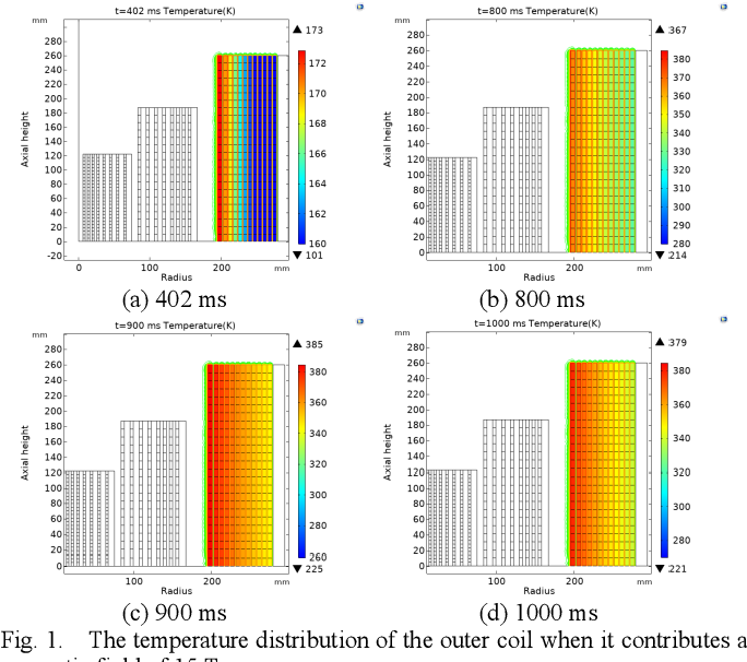
The output of such a simulation is a complete temperature map $T (r, t)$ . The image below shows the result of a sophisticated 2D finite element simulation (a more advanced numerical technique), illustrating the temperature distribution in a coil at several moments in time.

Temperature Distribution in a Pulsed Magnet Coil Over Time — Temperature distribution in a pulsed magnet coil at different times during and after the pulse: (a) 402 ms, (b) 800 ms, (c) 900 ms, (d) 1000 ms. This visualization is precisely what we aim to calculate with numerical methods, showing where and when the hotspots occur.

Test your understanding!

In our finite difference update equation, we assumed material properties like thermal conductivity $k$ and electrical resistivity $ρ_{e}$ were constant. In reality, they both depend strongly on temperature, i.e., $k = k (T)$ and $ρ_{e} = ρ_{e} (T)$ .

How would you modify the numerical simulation process to account for temperature-dependent properties? Where in the calculation loop would this change be implemented?

Show answer

You would need to update the material properties at each time step for each discrete element, based on its current temperature.

The modification would happen inside the main time-stepping loop, just before you calculate the new temperatures. The process for each time step would look like this:

You have the current temperature profile $T_{i} (t)$ for all shells $i$ .
For each shell $i$ , look up or calculate the material properties corresponding to its current temperature: $k_{i} = k (T_{i} (t))$ and $ρ_{e, i} = ρ_{e} (T_{i} (t))$ . This is typically done using a lookup table or a polynomial function fitted to experimental data.
Calculate the current heat generation using the updated resistivity: $e_{g e n, i} (t) = ρ_{e, i} J (t)^{2}$ .
Apply the finite difference update rule. Since $k$ now varies with position (because $T$ does), it cannot be pulled out of the spatial derivative. The term $\nabla \cdot (k \nabla T)$ needs to be discretized carefully. A common approach for the 1D term $\frac{1}{r} \frac{\partial}{\partial r} (r k \frac{\partial T}{\partial r})$ is to evaluate $k$ at the interfaces between shells (e.g., $k_{i + 1/2}$ ) to calculate the heat flux between them.
This gives you the new temperature profile, $T_{i} (t + Δ t)$ , and the process repeats.

This makes the problem non-linear, but it is straightforward to implement in a numerical code and is essential for accurate modeling of high-field magnets where temperature can change by hundreds of Kelvin.

Conclusion

Today, we've bridged the gap between the theoretical heat diffusion equation and its practical application in magnet design. While analytical solutions provide insight, we've seen that numerical methods like the Finite Difference Method are the essential tools for obtaining accurate temperature profiles in realistic scenarios.

Key Takeaways:

Solving the heat diffusion PDE requires specifying the equation, initial conditions, and boundary conditions.
Analytical solutions are limited to highly simplified cases. For practical magnet design, numerical methods are indispensable.
The Finite Difference Method (FDM) discretizes the conductor in space and time, turning the PDE into an iterative algebraic update rule.
The simulation process involves a heating phase (with a non-zero $e_{g e n}$ term) and a cooling phase ( $e_{g e n} = 0$ ), allowing for the calculation of the full temperature history $T (r, t)$ .
This method allows for the inclusion of realistic effects like time-varying currents and temperature-dependent material properties.

Next Lesson Preview:
In this lesson, we saw how temperature profiles evolve. You may have noticed in the simulations that for very short pulses, the heat doesn't have time to move far from where it was generated. For longer pulses, it diffuses significantly. In our next lesson, we will formalize this observation by introducing the concept of thermal diffusion length. We will learn to estimate this length to determine whether heating is adiabatic or quasi-steady for different pulse durations, providing a powerful rule of thumb for quick analysis without running a full simulation.

Recommended resources