Heat Diffusion in Joule-Heated Conductors

Hello! Welcome to the seventh module of our course.

In the last few lessons, we focused entirely on the immense mechanical forces generated within a pulsed magnet and the sophisticated structures required to contain them. We've tackled radial hoop stress and axial compression, completing the conceptual design of the magnet's mechanical support. However, as previewed, every powerful pulse deposits a massive amount of heat into the coil windings in mere milliseconds. Managing this thermal load is just as critical as managing the mechanical stress.

Today, we shift our focus from mechanics to thermodynamics. Our objective is to derive the heat diffusion equation for a conductor with internal Joule heating to model temperature evolution. This equation is the fundamental tool for predicting how a coil's temperature changes during and after a pulse. Mastering this derivation will provide the theoretical foundation for all thermal management analysis that follows.

1. The Foundation: Conservation of Energy

At its heart, the heat diffusion equation is a mathematical statement of the law of conservation of energy applied to a small volume of material. In words, the principle is straightforward:

The rate at which thermal energy changes inside a control volume is equal to the net rate of heat flowing into the volume through its boundaries, plus the rate at which heat is generated inside the volume.

Let's begin by watching a clear, first-principles derivation of this concept for a simple one-dimensional rod. This will establish the core ideas of energy balance, heat flux, and the role of material properties.

Deriving the Heat Equation: A Parabolic Partial Differential Equation for Heat Energy Conservation

This video from Steve Brunton provides an excellent conceptual and mathematical walkthrough of deriving the 1D heat equation from the principle of energy conservation.

Please watch from the beginning to 09:58. Focus on how he translates the verbal conservation law into a mathematical expression involving three key terms: a rate of change of heat energy, a heat flux term, and a heat generation term.

As the video explains, we can write the energy balance for a small volume element as:

\frac{\partial E _{s t or e d}}{\partial t} = (Q_{in} - Q_{o u t}) + E_{g e n}

Our task is to find mathematical expressions for each of these terms for a conductor in a magnet.

2. Formulating the Terms for a Conductor

Let's build the equation piece by piece, considering a small volume element of the conductor. For the general case, we can imagine a small rectangular volume element with sides $Δ x$ , $Δ y$ , and $Δ z$ .

General Heat Conduction Equation Derivation in Rectangular Coordinates — This diagram illustrates the energy balance on a small rectangular volume element. Heat enters and leaves through each face (the Q terms), while energy is generated internally (E_gen). The balance of these terms dictates the change in the element's stored energy.

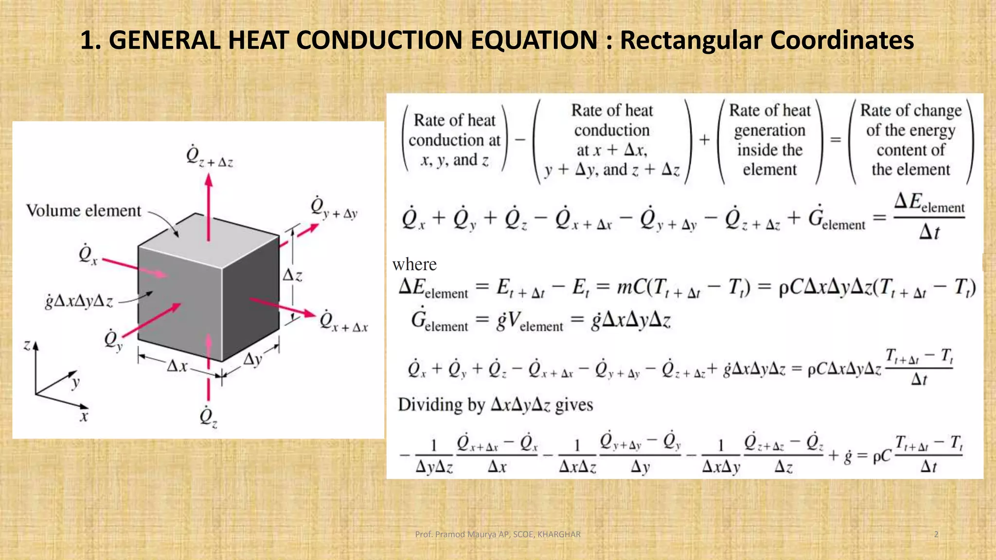
2.1. Stored Thermal Energy

The amount of thermal energy stored in the volume element depends on its mass and temperature. The rate of change of this energy is determined by the material's density $ρ$ (kg/m³) and its specific heat capacity $c$ (J/kg·K).

The rate of change of stored energy per unit volume is:

\frac{1}{V} \frac{\partial E _{s t or e d}}{\partial t} = ρ c \frac{\partial T}{\partial t}

where $T (x, y, z, t)$ is the temperature. This term represents the thermal inertia of the material.

2.2. Internal Heat Generation: Joule Heating

This is the term that makes our derivation specific to a current-carrying conductor. When current flows through a resistive material, electrical energy is converted into thermal energy. This is Joule heating. While the video referred to a generic source term q(x,t), in our case, this source is very specific.

The rate of heat generation per unit volume, which we'll call $e_{g e n}$ (in W/m³), is given by:

e_{g e n} = J \cdot E

where $J$ is the current density (A/m²) and $E$ is the electric field. Using Ohm's law in its vector form, $E = ρ_{e} J$ , where $ρ_{e}$ is the electrical resistivity (Ω·m), this becomes:

e_{g e n} = ρ_{e} J^{2}

For a pulsed magnet, the current density $J$ is a function of time, $J (t)$ , so the heat generation term will also be time-dependent.

The following resource provides a formal definition of the heat generation term and gives a clear example.

HEAT CONDUCTION EQUATION

The textbook 'HEAT CONDUCTION EQUATION' gives a precise definition of the heat generation term and its units, using the familiar example of electrical resistance heating.

Please read the section titled 'Heat Generation' (pages 68-69). Pay close attention to how the rate of heat generation per unit volume, e_gen, is defined and how it relates to electrical power.

2.3. Net Heat Conduction: Fourier's Law

Heat flows from hotter regions to colder regions. The mathematical description of this is Fourier's Law of Heat Conduction. It states that the heat flux vector $q^{''}$ (W/m²), which represents the rate of heat flow per unit area, is proportional to the negative gradient of the temperature:

q^{''} = - k \nabla T

Here, $k$ is the thermal conductivity of the material (W/m·K), which measures how well it conducts heat. The negative sign ensures that heat flows "downhill" from high to low temperature.

The net rate of heat conduction into a volume is given by the negative divergence of the heat flux vector, $- \nabla \cdot q^{''}$ . Substituting Fourier's Law gives:

Net Conduction Rate = - \nabla \cdot (- k \nabla T) = \nabla \cdot (k \nabla T)

3. Assembling the General Heat Diffusion Equation

Now we combine the three terms into our energy balance equation. All terms are expressed per unit volume:

Rate of Energy Storage ρ c \frac{\partial T}{\partial t} = Net Heat Conduction \nabla \cdot (k \nabla T) + Internal Heat Generation e_{g e n}

This is the general heat diffusion equation for a medium with internal heat generation. It's a second-order partial differential equation that governs the temperature distribution $T (x, y, z, t)$ .

For many practical cases, the thermal conductivity $k$ can be treated as a constant (though in reality it depends on temperature). In this case, it can be pulled out of the divergence operator:

ρ c \frac{\partial T}{\partial t} = k \nabla^{2} T + e_{g e n}

where $\nabla^{2}$ is the Laplacian operator. Dividing by $ρ c$ , we get the standard form:

\frac{\partial T}{\partial t} = \frac{k}{ρ c} \nabla^{2} T + \frac{e _{g e n}}{ρ c}

We define the term $α = \frac{k}{ρ c}$ as the thermal diffusivity (m²/s). This important property measures how quickly a material responds to changes in temperature.

So, the final equation is:

\frac{\partial T}{\partial t} = α \nabla^{2} T + \frac{e _{g e n}}{ρ c}

Equation in Cylindrical Coordinates

Since magnet windings are essentially cylindrical, it's most useful to express this equation in cylindrical coordinates $(r, ϕ, z)$ . Assuming temperature varies only with radius $r$ and time $t$ (a good approximation for a long, uniform wire), the Laplacian $\nabla^{2} T$ simplifies, and the equation becomes:

\frac{\partial T}{\partial t} = α (\frac{\partial ^{2} T}{\partial r ^{2}} + \frac{1}{r} \frac{\partial T}{\partial r}) + \frac{e _{g e n}}{ρ c}

This is the form of the heat diffusion equation you will most often use when modeling the thermal behavior of a conductor in a coil.

The following resource provides a rigorous step-by-step derivation for different coordinate systems, confirming the result we've just built.

HEAT CONDUCTION EQUATION

To see the formal, step-by-step derivation in different coordinate systems, let's return to the 'HEAT CONDUCTION EQUATION' textbook.

Please review Section 2-2, 'ONE-DIMENSIONAL HEAT CONDUCTION EQUATION', and Section 2-3, 'GENERAL HEAT CONDUCTION EQUATION' (pages 69-77). In Section 2-2, focus on the derivation for a 'Long Cylinder'. Trace how the energy balance on a cylindrical shell element (Eq. 2-18) leads to the final 1D transient equation (Eq. 2-26), which includes the e_gen term. In Section 2-3, look at the general equation in 3D for cylindrical coordinates (Eq. 2-43). This confirms how our general vector equation maps to the specific coordinate system relevant to our work.

Test your understanding!

Consider a very long, solid cylindrical conductor made of copper. During a brief pulse, it carries a high, constant current density $J_{0}$ . We are interested in the temperature at the very center of the wire ( $r = 0$ ). At the beginning of the pulse ( $t = 0$ ), the entire wire is at a uniform temperature $T_{ambi e n t}$ .

For this specific scenario, how does the heat diffusion equation simplify? What does this tell you about the initial rate of temperature rise at the center of the wire?

(Hint: At $r = 0$ , what can you say about the term $\frac{1}{r} \frac{\partial T}{\partial r}$ ? Think about the temperature profile—it must be smooth and symmetric at the center.)

Show answer

The full equation is:

\frac{\partial T}{\partial t} = α (\frac{\partial ^{2} T}{\partial r ^{2}} + \frac{1}{r} \frac{\partial T}{\partial r}) + \frac{ρ _{e} J _{0}^{2}}{ρ c}

Simplifying the conduction term: Due to the radial symmetry of the problem, the temperature profile must be flat at the center, meaning the temperature gradient is zero: $\frac{\partial T}{\partial r}_{r = 0} = 0$ . The term $\frac{1}{r} \frac{\partial T}{\partial r}$ is an indeterminate $0/0$ form at $r = 0$ . Using L'Hôpital's rule, this limit becomes $\frac{\partial ^{2} T}{\partial r ^{2}}_{r = 0}$ . Therefore, at $r = 0$ , the conduction term simplifies:
$(\frac{\partial ^{2} T}{\partial r ^{2}} + \frac{1}{r} \frac{\partial T}{\partial r})_{r = 0} = \frac{\partial ^{2} T}{\partial r ^{2}}_{r = 0} + \frac{\partial ^{2} T}{\partial r ^{2}}_{r = 0} = 2 \frac{\partial ^{2} T}{\partial r ^{2}}_{r = 0}$
So, at the center, the equation is:
$\frac{\partial T}{\partial t}_{r = 0} = 2 α \frac{\partial ^{2} T}{\partial r ^{2}}_{r = 0} + \frac{ρ _{e} J _{0}^{2}}{ρ c}$
Initial rate of temperature rise: At the very instant the pulse starts ( $t = 0$ ), no heat has had time to conduct away from any point. The temperature is still uniform at $T_{ambi e n t}$ , so the temperature gradient and its derivatives are zero everywhere. Therefore, $\frac{\partial ^{2} T}{\partial r ^{2}}_{t = 0} = 0$ .

The conduction term vanishes at $t = 0$ , and the equation simplifies dramatically to:
$\frac{\partial T}{\partial t}_{t = 0} = \frac{ρ _{e} J _{0}^{2}}{ρ c}$
This tells us that, initially, the temperature everywhere in the wire (including the center) rises at a rate determined purely by the Joule heating and the material's volumetric heat capacity ( $ρ c$ ). The heat has not yet had time to redistribute itself via conduction. This initial phase is known as adiabatic heating.

Conclusion

In this lesson, we have meticulously derived one of the most important equations in thermal engineering from the fundamental principle of energy conservation. You are now equipped with the theoretical tool needed to model the temperature inside a conductor subjected to intense heating.

Key Takeaways:

The heat diffusion equation is a mathematical statement of the conservation of energy.
It balances the rate of energy storage ( $ρ c \frac{\partial T}{\partial t}$ ), net heat conduction ( $\nabla \cdot (k \nabla T)$ ), and internal heat generation ( $e_{g e n}$ ).
For a current-carrying conductor, the internal heat generation term is Joule heating, given by $e_{g e n} = ρ_{e} J (t)^{2}$ .
The material property $α = k / (ρ c)$ , called thermal diffusivity, determines how quickly temperature changes propagate through the material.
For magnet coils, the equation is most practically expressed in cylindrical coordinates.

Next Lesson Preview:
Having derived the governing equation, our next step is to solve it. In the next lesson, we will apply the heat diffusion equation to calculate the temperature profile in a conductor during and after a current pulse. We will investigate two important regimes: the very short pulse limit (adiabatic heating) and longer pulses where thermal diffusion plays a significant role. This will allow us to predict the peak temperature rise in a coil, a critical parameter for preventing burnout.

Recommended resources