Thermal Equilibrium in Pulsed Magnets

Hello! Welcome to the final lesson in our module on Thermal Management and Cooling.

In our last session, we analyzed the complex interplay of thermal and electromagnetic stresses that arise during a single, powerful current pulse. We saw how non-uniform heating induces stresses that superimpose on the primary Lorentz force-driven stresses. Today, we shift our focus from the effects of a single pulse to the behavior of a magnet under repetitive operation, a standard scenario in research facilities like LNCMI.

This lesson is dedicated to the learning outcome: Calculate the thermal equilibrium temperature in a repetitively pulsed magnet by balancing Joule heating with inter-pulse cooling. We will develop a model to understand how a magnet's temperature evolves over many pulse cycles and settles into a stable operating condition. This concept is crucial for determining the maximum sustainable repetition rate of an experiment, a key operational parameter that directly impacts data acquisition speed.

1. The Concept of Thermal Equilibrium

When a magnet is pulsed repeatedly, each pulse injects a quantum of heat, $Q_{in}$ , into the windings. Between pulses, the cooling system works to remove this heat. Initially, if the cooling is not fast enough to remove all the heat before the next pulse arrives, the magnet's average temperature will begin to rise.

As the magnet's temperature increases, the rate of heat dissipation to the surroundings (which is proportional to the temperature difference) also increases. This process continues until the magnet reaches a state of thermal equilibrium, where the average power from Joule heating is exactly balanced by the average power removed by the cooling system.

The image below illustrates this process. The bottom plot shows repetitive power pulses. The top plot shows the corresponding temperature of the component. Notice how the temperature oscillates—rising during the pulse, falling between pulses—but the average temperature climbs and then stabilizes. This stable average temperature is the thermal equilibrium temperature.

Temperature Evolution in Repetitively Pulsed Systems — Evolution of temperature in a component subjected to repetitive power pulses. The temperature rises during each pulse and falls during the cooling interval, eventually settling into a stable oscillation around an equilibrium average temperature.

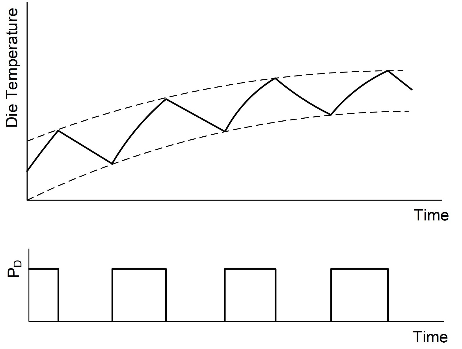
At equilibrium, the temperature profile becomes periodic. The goal of our analysis is to predict this final equilibrium state, specifically the average, peak ( $T_{p e ak}$ ), and minimum ( $T_{min}$ ) temperatures the coil will experience.

2. The Heat Balance Equation

The fundamental condition for thermal equilibrium is that over one full cycle (one pulse plus one cooling interval), the energy input equals the energy output.

Let:

$Q_{in}$ be the total Joule heat generated during one pulse (duration $t_{p u l se}$ ).
$⟨ P_{coo l} ⟩$ be the average cooling power over one repetition period.
$t_{r e p}$ be the repetition period (the time from the start of one pulse to the start of the next).

The equilibrium condition is:
$Average Heating Power = Average Cooling Power$
$\frac{Q _{in}}{t _{r e p}} = ⟨ P_{coo l} ⟩$

To solve this, we need models for both $Q_{in}$ and $⟨ P_{coo l} ⟩$ .

Modeling Joule Heating ( $Q_{in}$ )

From our previous work, the heat generated during a pulse is the integral of the instantaneous power:
$Q_{in} = \int_{0}^{t_{p u l se}} I (t)^{2} R (T (t)) d t$
A key complication is that the coil's resistance, $R$ , is a function of its temperature, $T$ . Since the magnet is operating at an elevated equilibrium temperature, its resistance will be significantly higher than at room temperature. For copper, this relationship is nearly linear over a moderate temperature range.

Modeling Cooling ( $P_{coo l}$ )

The cooling process is often modeled by Newton's law of cooling, where the rate of heat loss is proportional to the temperature difference between the object and its surroundings:
$P_{coo l} (t) = h A (T (t) - T_{ambi e n t})$
Here, $h$ is the heat transfer coefficient, $A$ is the cooling surface area, and $T_{ambi e n t}$ is the temperature of the coolant (e.g., air, water, or liquid nitrogen).

Since the coil's temperature $T (t)$ varies during the cooling period, the average cooling power $⟨ P_{coo l} ⟩$ is approximately $h A (T_{e q} - T_{ambi e n t})$ , where $T_{e q}$ is the average equilibrium temperature of the coil.

3. Calculating the Equilibrium Temperature: An Analytical Approach

Let's combine these models into a single equation. We can approximate the resistance during the pulse using its value at the average equilibrium temperature, $R (T_{e q})$ .

Our heat balance equation becomes:
$\frac{R ( T _{e q} )}{t _{r e p}} \int_{0}^{t_{p u l se}} I (t)^{2} d t = h A (T_{e q} - T_{ambi e n t})$

The integral $\int_{0}^{t_{p u l se}} I (t)^{2} d t$ depends only on the current pulse shape and magnitude. Let's call this the pulse "action integral," $S_{I}$ . The resistance can be expressed using a linear model: $R (T_{e q}) = R_{0} (1 + β (T_{e q} - T_{0}))$ , where $R_{0}$ is the resistance at a reference temperature $T_{0}$ and $β$ is the temperature coefficient of resistance.

Substituting this in, we get:
$\frac{S _{I}}{t _{r e p}} R_{0} (1 + β (T_{e q} - T_{0})) = h A (T_{e q} - T_{ambi e n t})$

This is a linear equation in $T_{e q}$ , which you can solve to find the average equilibrium temperature. Given your background, you can see how this provides a powerful, first-order estimate for a magnet's operating temperature based on its material properties, pulse characteristics, and cooling system efficiency.

Test your understanding!

A copper coil has a resistance of 50 mΩ at 20°C. Its temperature coefficient of resistance is $β = 0.004 K^{- 1}$ . The coil is pulsed with a repetition time $t_{r e p} = 60$ s. The "action integral" for the pulse is $S_{I} = 2 \times 1 0^{9} A^{2} s$ . The cooling system is characterized by $h A = 10 W/K$ , and the ambient temperature is 20°C.

Estimate the average equilibrium temperature $T_{e q}$ of the coil.

Show answer

We start with the heat balance equation:
$\frac{S _{I}}{t _{r e p}} R_{0} (1 + β (T_{e q} - T_{0})) = h A (T_{e q} - T_{ambi e n t})$
Here, $S_{I} = 2 \times 1 0^{9} A^{2} s$ , $t_{r e p} = 60 s$ , $R_{0} = 0.05 Ω$ , $β = 0.004 K^{- 1}$ , $T_{0} = 2 0^{\circ} C$ , $h A = 10 W/K$ , and $T_{ambi e n t} = 2 0^{\circ} C$ .

First, calculate the average heating power factor:
$P_{a v g, h e a t_f a c t or} = \frac{S _{I} R _{0}}{t _{r e p}} = \frac{( 2 \times 1 0 ^{9} A ^{2} s ) ( 0.05 Ω )}{60 s} \approx 1666.7 W$

Now, substitute this into the equation:
$1666.7 \cdot (1 + 0.004 \cdot (T_{e q} - 20)) = 10 \cdot (T_{e q} - 20)$
Let $Δ T = T_{e q} - 20$ .
$1666.7 \cdot (1 + 0.004 \cdot Δ T) = 10 \cdot Δ T$
$1666.7 + 6.667 \cdot Δ T = 10 \cdot Δ T$
$1666.7 = (10 - 6.667) \cdot Δ T$
$1666.7 = 3.333 \cdot Δ T$
$Δ T = \frac{1666.7}{3.333} \approx 500 K$
So, $T_{e q} = 20 + 500 = 52 0^{\circ} C$ .

This extremely high temperature indicates that the proposed pulsing scheme is not sustainable for this coil and cooling system. The coil would likely melt or its insulation would fail long before reaching this temperature. This demonstrates how this calculation is a critical safety and design check.

4. A Practical Case Study: The "Foil Coil"

The simplified model above is a great start. To see how these concepts play out in a real-world magnet, let's examine a case study from a paper describing a magnet designed at LNCMI.

A novel pulsed magnet for magnetic linear birefringence ...

The paper 'A novel pulsed magnet for magnetic linear birefringence...' describes the design and testing of a unique room-temperature pulsed magnet. The discussion on its thermal performance provides a perfect real-world example of the balance between heating and cooling.

Please read the section titled 'Repetition rate' that starts on page 6. It begins with the sentence 'Repetition rate will be important to perform an experiment where hundreds of pulses will be necessary.' Focus on: Temperature Measurement: How the authors use the measured resistance and the linear temperature dependence of copper resistivity to deduce the coil's temperature. Operational Limits: The maximum average temperature they set (60°C) to preserve the magnet's integrity. Cooling Dynamics: The description of the multi-stage cooling process and the graph in Fig. 9 showing exponential-like decay. This highlights that our simple single-exponential model is an approximation of a more complex heat diffusion problem. The Final Balance: The key conclusion: 'A final temperature fixed at 60°C leads to a cooling duration of the magnet before another pulse at 12.5 T of about 50 minutes.' This is a direct statement of the calculated balance between heating and cooling for a specific operational target.

This paper provides several crucial insights. Firstly, it validates our approach of using resistance to monitor temperature. Secondly, it reveals the complexity of real-world cooling, which involves heat diffusing through multiple layers (copper, Kapton insulation, Zylon reinforcement) with different thermal properties, leading to multiple time constants.

Most importantly, it provides a very practical design constraint. The paper also makes this statement: "Duty cycle will increase proportionally to the inverse of the square of the magnetic ﬁeld." Let's quickly verify this.

Joule heating $Q_{in}$ is proportional to $\int I^{2} d t$ .
Since the magnetic field $B$ is proportional to the current $I$ , $Q_{in} \propto B_{p e ak}^{2}$ .
The average heating power is $P_{h e a t} = Q_{in} / t_{r e p} \propto B_{p e ak}^{2} / t_{r e p}$ .
The average cooling power $P_{coo l}$ is determined by the target equilibrium temperature, which is fixed (e.g., at 60°C). So, $P_{coo l}$ is constant.
At equilibrium, $P_{h e a t} = P_{coo l}$ , so $B_{p e ak}^{2} / t_{r e p} = constant$ .
This implies that the repetition time $t_{r e p} \propto B_{p e ak}^{2}$ .

This is a fundamental scaling law in pulsed magnet operation: to double the field, you must wait four times as long between pulses to maintain the same operating temperature.

5. An Alternative View: Thermal Impedance

In electrical and thermal engineering, the concept of thermal impedance, $Z_{θ}$ , is often used. It's defined by the relation $Δ T = P \cdot Z_{θ}$ , analogous to Ohm's law. For repetitive pulses, the effective thermal impedance depends on the pulse duration and the duty cycle ( $D = t_{p u l se} / t_{r e p}$ ).

Normalized Thermal Impedance vs. Pulse Duration for Different Duty Cycles — Normalized thermal impedance as a function of pulse duration for a single pulse and for various duty cycles. For repetitive pulses, the effective thermal impedance is higher, leading to a higher average temperature for the same power.

This graph shows that for a given pulse duration, a higher duty cycle (i.e., less cooling time) results in a higher effective thermal impedance. This is another way of expressing that the average temperature increases as the repetition rate goes up. The "single pulse" curve represents the temperature rise from a single event, while the curves for D > 0 represent the higher, steady-state temperature oscillations at thermal equilibrium.

Conclusion

Today, we've established the framework for analyzing the thermal performance of a repetitively pulsed magnet. By balancing average heating and cooling power, we can predict the stable operating temperature, which in turn dictates the maximum sustainable repetition rate—a critical parameter for any experiment.

Key Takeaways:

Thermal Equilibrium: A repetitively pulsed magnet reaches thermal equilibrium when the average Joule heating power per cycle equals the average cooling power.
Heat Balance Equation: The equilibrium temperature $T_{e q}$ can be estimated by solving the equation $\frac{S _{I} R ( T _{e q} )}{t _{r e p}} = h A (T_{e q} - T_{ambi e n t})$ .
Repetition Rate Scaling: For a fixed operating temperature, the required repetition time $t_{r e p}$ scales with the square of the peak magnetic field ( $t_{r e p} \propto B_{p e ak}^{2}$ ).
Practical Limits: The equilibrium temperature must be kept below a critical threshold (e.g., 60-80°C for the Foil Coil) to protect the coil's insulation and mechanical integrity.

Next Lesson Preview:
With this lesson, we conclude our deep dive into the thermal and mechanical analysis of pulsed magnets. We now have a solid theoretical understanding of the fundamental forces, stresses, and thermal limits that govern magnet design. In our next module, we will transition from theory to practice. We'll begin by addressing the very first step in manufacturing a high-field coil: precision winding techniques. We will explore how the idealized cylindrical geometries we have been analyzing are meticulously constructed in the real world to ensure optimal performance and reliability.

Recommended resources