Log Returns: Calculation & Visualization

Welcome back. In our first lesson, we explored the hierarchy of financial data, culminating in the creation of OHLCV bars from raw trades. You learned that the closing price series from this data is a common starting point for analysis. Today, we will perform the first and most crucial transformation on that price series: converting it into log returns.

This lesson directly addresses the learning outcome of computing and visualizing log returns. For almost any quantitative model you build, from simple signal analysis to complex deep learning predictors, you will work with returns, not raw prices. We'll investigate why this is the case, distinguish between simple and log returns, and establish why log returns are the standard for time-series modeling in finance. This process is the first step in engineering features from raw market data, a concept that should be familiar from your machine learning projects.

Why Work with Returns?

A raw price series of a stock, say from $10 to $110 over a decade, has a clear upward trend. In statistical terms, its mean is not constant over time, making it non-stationary. Most statistical models, and by extension many machine learning models, assume stationarity—that the statistical properties of the series (like mean and variance) do not change over time.

By converting prices to returns, we look at the percentage change from one period to the next. This new series tends to be much more stationary, fluctuating around a mean close to zero. This transformation makes the data much more amenable to modeling.

There are two common ways to calculate returns: simple returns and log returns. Let's start with the more intuitive one.

Simple Returns: The Investor's Perspective

The simple return ( $R_{t}$ ) is exactly what it sounds like: the percentage change in price over one period.

R_{t} = \frac{P _{t} - P _{t - 1}}{P _{t - 1}} = \frac{P _{t}}{P _{t - 1}} - 1

While intuitive, simple returns have a major drawback for time-series analysis: they are not additive over time. A simple example illustrates this perfectly.

Simple Returns vs Log Returns : WHAT TO CHOOSE?

The video "Simple Returns vs Log Returns" provides a fantastic numerical example to start us off.

Please watch the introductory segment from the beginning to the end of the example. The presenter shows that if a stock goes from $100 to $200 (+100% simple return) and then back to $100 (-50% simple return), simply adding the returns gives a misleading +50%, whereas the net change is clearly 0%.

As the video shows, to correctly calculate the total return over multiple periods using simple returns, you must compound them:

1 + R_{total} = (1 + R_{1}) \times (1 + R_{2}) \times \dots \times (1 + R_{n})

This multiplicative property is cumbersome for modeling. We want a representation where combining returns over time is as simple as adding them up.

Log Returns: The Modeler's Choice

Log returns (or continuously compounded returns, $r_{t}$ ) solve the aggregation problem. The log return is defined as the natural logarithm of the price ratio.

r_{t} = ln (\frac{P _{t}}{P _{t - 1}}) = ln (P_{t}) - ln (P_{t - 1})

The magic of logarithms transforms the multiplicative relationship into an additive one. The total log return over $N$ periods is simply the sum of the individual per-period log returns:

r_{total} = t = 1 \sum N r_{t} = r_{1} + r_{2} + \dots + r_{N}

This time-additive property is incredibly useful. It allows us to calculate multi-period returns by simple summation, which simplifies many statistical procedures.

Calculating and Comparing in Python

Now let's see how this is done in practice. You'll find that with pandas and numpy, these calculations are trivial. The following video demonstrates how to fetch data and compute both simple and log returns.

Python for Finance: Are stock returns normally distributed?

The video "Python for Finance: Are stock returns normally distributed?" provides a clear, code-along demonstration.

Watch these specific segments to see the concepts in action: Calculating Simple Returns: Start at this section to see how to use the .pct_change() method in pandas. Calculating Log Returns: Jump to this part to see the standard numpy implementation: np.log(df.close / df.close.shift(1)). The Additive Property: Finally, watch from this demonstration. It shows how the mean of log returns can be used to accurately reconstruct the final price over the period, proving their additive utility, whereas the mean of simple returns cannot be used this way.

The key Python snippets to add to your toolkit are:

Simple Returns: simple_returns = prices.pct_change()
Log Returns: log_returns = np.log(prices / prices.shift(1))

The Connection Between Simple and Log Returns

How are these two measures related? The formula is straightforward:

r_{t} = ln (\frac{P _{t}}{P _{t - 1}}) = ln (1 + R_{t})

For small values of $x$ , the Taylor series expansion for $ln (1 + x)$ is $x - \frac{x ^{2}}{2} + \dots$ . This means that for small returns, which are very common for daily financial data, the log return is approximately equal to the simple return: $r_{t} \approx R_{t}$ .

On the left, this plot compares the functions f(x) = x (representing simple returns) and f(x) = log(1+x) (representing log returns). Notice how the two curves are almost identical for small values of x near zero, but diverge as x gets larger. The plot on the right is a Quantile-Quantile (QQ) plot, which we will explore in a future lesson.

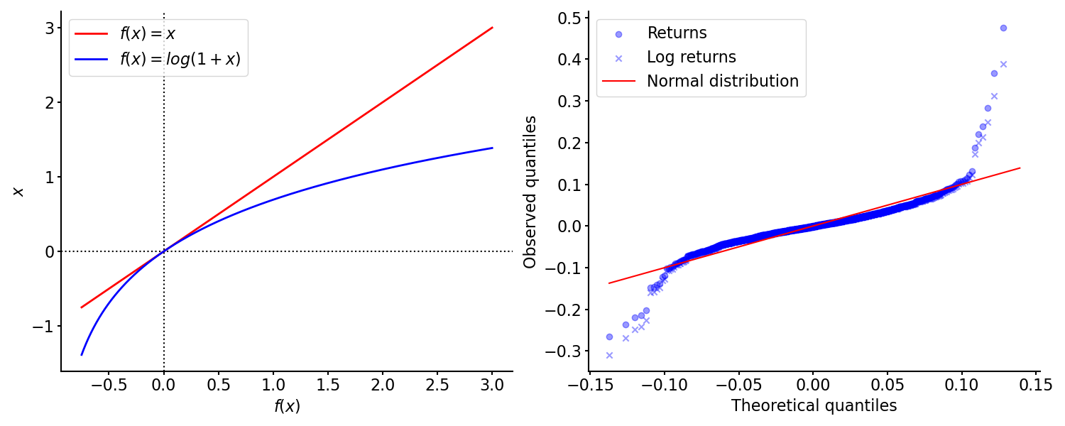
This approximation is important. It tells us that for high-frequency data, the choice between simple and log returns might not dramatically change results. However, as the return magnitude increases (e.g., for weekly/monthly returns or during market crashes), the difference becomes significant, and the additive property of log returns makes them far superior for modeling.

This article provides a great summary of the key properties.

Data Handling & Visualization: Python for Quant Finance ...

This article from mbrenndoerfer.com offers a clear technical breakdown of the two return types.

Read the section Computing Returns. Focus on the distinction it makes: Simple returns aggregate across assets in a portfolio. If you have a portfolio of 50% Asset A and 50% Asset B, the portfolio's simple return is 0.5 * R_A + 0.5 * R_B. Log returns aggregate across time for a single asset. For most time-series prediction tasks, you will be concerned with aggregation across time, making log returns the default choice.

Visualizing the Distribution of Returns

The final part of our objective is to visualize the returns we've calculated. A histogram is the most common way to do this. It shows us the frequency of returns of different magnitudes and gives us a first look at the underlying probability distribution.

Let's return to the QuantPy video to see how to generate this plot.

Python for Finance: Are stock returns normally distributed?

The video provides a simple way to plot a histogram of the log returns.

Please watch the short segment from plotting the histogram. The presenter uses log_returns.plot(kind='hist') to quickly generate the visualization.

When you generate such a histogram, you will typically see a distribution that is sharply peaked at zero and has values extending out in both the positive and negative directions. It might look like a normal (Gaussian) distribution, but on closer inspection, you'll often find it's not quite a perfect match.

Conclusion

In this lesson, we made the crucial transition from prices to returns. You now understand the "why" and "how" of this fundamental preprocessing step.

Here are the key takeaways:

We use returns instead of prices for modeling because returns are more stationary.
Simple returns ( $(P_{t} / P_{t - 1}) - 1$ ) are intuitive but not additive over time, making them ill-suited for most time-series analysis.
Log returns ( $ln (P_{t} / P_{t - 1})$ ) are time-additive, a convenient property that makes them the standard for quantitative finance.
The essential Python commands are prices.pct_change() for simple returns and np.log(prices / prices.shift(1)) for log returns.
For small percentage changes, simple and log returns are nearly identical.

We concluded by visualizing the distribution of log returns. This distribution has several interesting and consistent properties, regardless of the asset or market. In our next lesson, we will formally explore these "stylized facts" of financial returns, including their "fat tails" and "volatility clustering," and see how to test for them.

Recommended resources