Welcome to the first lesson of your preparatory course for the Algo Arena competition. Given your strong background in machine learning and software engineering, you're already equipped with many of the core skills needed in quantitative finance. Our goal over the next eight days is to bridge the gap between your existing expertise and the specific domain knowledge of financial markets.
This first lesson focuses on the raw material of any quantitative strategy: market data. In the competition, you'll be presented with a dataset and a problem. Knowing precisely what that data represents, how it was generated, and its inherent limitations is the critical first step before any modeling or analysis can begin. We will start with the most fundamental and granular representation of market activity—the order book—and progressively build up to the aggregated data formats you are more likely to encounter, such as OHLCV bars.
The Foundation: The Limit Order Book
At any given moment, a market for a financial instrument is defined by the intentions of its participants. The Limit Order Book (LOB) is the data structure that electronically stores all active buy and sell orders for a specific asset. Think of it as a real-time, double-sided priority queue, where orders are prioritized first by price and then by time.
To get a clear picture of how this works, let's start with a video that explains the concept from the ground up.
Understand the orderbook like a quant
The video "Understand the orderbook like a quant" provides an excellent, intuitive introduction to the structure of the order book.
Please watch the following segments: What is an order book? this section will introduce the basic definition. Level 1 (L1) Data: This part explains the most important prices on the book: the best bid (the highest price a buyer is willing to pay) and the best ask (the lowest price a seller is willing to accept). Level 2 (L2) Data: This segment introduces the concept of market depth, showing the quantity of buy and sell orders at different price levels beyond just the best prices. As you watch, focus on understanding the distinction between the bid side (demand) and the ask side (supply), and how L2 data gives a more complete picture of market liquidity than L1 alone.
The difference between the best ask and the best bid is called the bid-ask spread. A narrow spread generally indicates high liquidity and a competitive market, while a wide spread can suggest the opposite. The total quantity of shares available at different price levels on the bid and ask sides constitutes the market's depth.
From Intentions to Actions: Trades and Quotes
The order book represents potential trades. An actual trade occurs when these intentions are met—specifically, when an incoming order is matched with a resting order on the book. This is often called "crossing the spread" or "taking liquidity."
The following short video from Udacity provides a clear, visual demonstration of how different types of orders interact with the order book to generate trades.
How orders affect the order book
This video, "How orders affect the order book," visually simulates the execution of trades and their impact on the available liquidity.
Watch these key examples: Market Buy Order: See how a simple buy order consumes liquidity from the ask side at the best available price. Limit Buy Order: Observe how a limit order is filled at or better than its specified price. Large Market Sell Order: Notice how a large order can "walk the book," consuming liquidity across multiple price levels and resulting in an average execution price. This phenomenon is known as slippage.
This leads us to our first two formal data types:
-
Tick-Level Trade Data: This is the most granular record of market activity. Each "tick" represents a single, executed trade, captured with its price, volume (size), and a precise timestamp. It's the ground truth of what has happened in the market.
-
Quote Data: This is a time-series record of the L1 order book information—specifically, the best bid and best ask prices, and usually the volume available at those prices. It gives you a view of the market's posted liquidity over time, but not what trades were actually filled.
The following article gives a concise definition of these data types.
Understanding Crypto Market Data: From Tick Trades to OHLCV and ...
This article from CoinAPI provides clear, snapshot-based examples of different market data types.
Please read the first two sections: Tick-Level Trades: Focus on the structure of the example table (Timestamp, Price, Amount). This is the raw log of executed transactions. Quotes: Note how this data includes separate entries for bid/ask prices and sizes. This represents the state of the top of the order book over time.
Aggregating for Analysis: OHLCV Data
While tick and quote data are essential for high-frequency trading and detailed microstructure analysis, they can be unwieldy for many other applications. The sheer volume of data is often too large, and the "noise" can obscure longer-term patterns.
For this reason, trade data is commonly aggregated into fixed time intervals, creating what is arguably the most recognized data format in finance: OHLCV bars.
- Open: The price of the first trade in the interval.
- High: The highest trade price in the interval.
- Low: The lowest trade price in the interval.
- Close: The price of the last trade in the interval.
- Volume: The total quantity of the asset traded during the interval.
These are often visualized as candlesticks or bars.
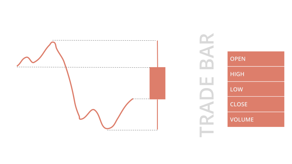
The process of creating OHLCV bars is a form of lossy compression. You gain a structured, fixed-size representation of price action, which is extremely useful for charting, backtesting, and training many types of models. However, you lose all information about what happened within the bar.
The following article explains OHLCV data in more detail.
OHLCV Data Explained: Real-Time Updates, WebSocket ...
This article provides a practical breakdown of OHLCV data, its construction, and its limitations.
Please focus on these sections: What is OHLCV?: This gives a high-level overview. How to Read OHLCV Data?: This section provides a concrete example of interpreting a single row of OHLCV data. Limitations of OHLCV Data: This is a crucial section. Understanding what information is lost during aggregation is key to avoiding flawed analysis.
The Hierarchy of Financial Data
To bring it all together, we can think of these data types as a hierarchy of abstraction, from raw intent to aggregated summary:
- Order Book (L2/L3): The complete state of all resting orders. This is the most comprehensive view but also the most complex.
- Quotes (L1): A time series of the best bid and ask. A high-frequency summary of the most relevant part of the order book.
- Trades (Ticks): The log of executed transactions. The ground truth of what was exchanged.
- OHLCV: Aggregated summaries of trades over time intervals. The most common format for historical analysis and many modeling approaches.
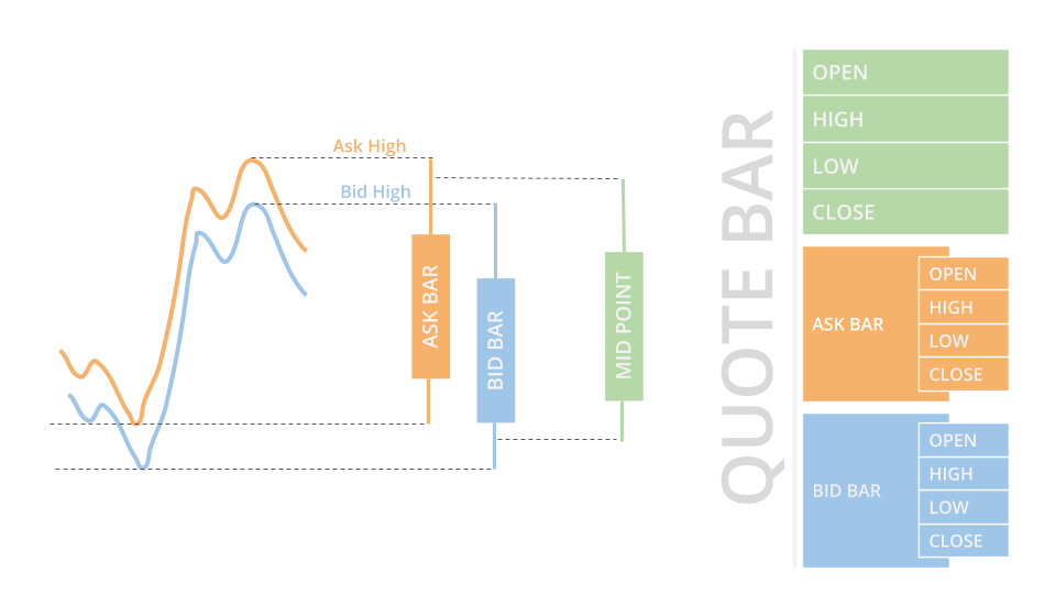
The choice of which data to use depends entirely on the problem you're trying to solve. For your competition, you might be given OHLCV data to predict future price movements, or you might receive tick data and need to simulate a trading strategy's execution, accounting for slippage. Knowing how they relate is fundamental.
The table in the Understanding Crypto Market Data article provides an excellent reference for this.
Understanding Crypto Market Data: From Tick Trades to OHLCV and ...
Let's revisit this article for its final summary table.
Review the table under the heading Quick Reference Guide. This table concisely maps different data types to common quantitative use cases. It's a great mental model to keep in mind.
Conclusion
In this lesson, we've deconstructed the primary forms of financial market data. You've seen that the dynamic order book is the source of all activity. From it, we derive a stream of trades (executed orders) and quotes (snapshots of the best prices). Finally, we saw how trades are aggregated into the ubiquitous OHLCV bars for higher-level analysis.
Understanding this data hierarchy is not just academic; it's a practical necessity. It informs how you interpret data, what features you can engineer, and what limitations your models might have.
In our next lesson, we will begin processing this data. We'll take a series of prices—like the closing prices from OHLCV data—and transform them into log returns. This is the standard first step in nearly all quantitative financial analysis, as returns have much more desirable statistical properties than raw prices.