Hello! Welcome to the first lesson in our second module on Single Machine Scheduling.
In the previous module, we built a strong foundation. We learned how to describe scheduling problems using standard notation, explored different objectives, and critically, we delved into computational complexity. You now know why some problems are considered "easy" (in P) while others, like the Flexible Job Shop Problem you're focusing on for your thesis, are "hard" (NP-hard).
Today, we transition from theory to practice by tackling one of the most fundamental "easy" problems in scheduling. This lesson will show you how a simple, elegant rule can provide a guaranteed optimal solution for a specific objective.
This lesson addresses the learning outcome: Apply the Shortest Processing Time (SPT) rule to minimize total completion time on a single machine.
While a single-machine environment is much simpler than an FJSP, mastering these basic models is essential. The principles of applying a rule, calculating performance metrics, and understanding optimality proofs are universal skills that you will build upon as we move to more complex flow shop and job shop environments.
1. The Single Machine Problem: Minimizing Total Completion Time
Let's start by formally defining our problem. We are in a single-machine environment where a set of n jobs is ready to be processed at time zero. Each job j has a known processing time, . Our goal is to find a sequence for these jobs that minimizes the total completion time, denoted as .
In the standard three-field notation we learned, this problem is written as **1 | | **.
- 1: A single machine.
- [empty]: Standard assumptions apply (e.g., all jobs available at time 0, no preemption).
- : The objective is to minimize the sum of the completion times of all jobs.
Minimizing total completion time is a common industrial objective. It's directly related to minimizing the average time jobs spend in the system and, by Little's Law, also minimizes the average work-in-process (WIP) inventory.
For a deeper look at the assumptions of this model and the importance of performance measures, please review the following text.
The following sections from the textbook 'Chapter 2' by Walter J. Böhm establish the context for our single-machine problems. They define the model, its assumptions, and the concept of 'regular performance measures', which justifies our focus on simple permutation schedules.
Read the following parts: Section 2.1 'The model and its assumptions'. Section 2.2 'The schedule and its outcome' (up to, but not including, 'Preemption'). Section 2.3 'Performance Measures' (up to, but not including, the recurrence formula C(i) = ...). Focus on understanding why, for an objective like total completion time, we only need to consider schedules without preemption or inserted idle time. This reduces the problem from an infinite number of possible schedules to a finite number (n!) of job permutations.
2. The Shortest Processing Time (SPT) Rule
The solution to the 1 | | ΣCj problem is astonishingly simple and intuitive. The optimal sequence is found by applying the Shortest Processing Time (SPT) rule:
To minimize the total completion time, process the jobs in non-decreasing order of their processing times.
This means you always process the shortest job available first, then the next shortest, and so on, until the longest job is processed last.
Let's see this rule in action. The following video provides a clear, step-by-step walkthrough of applying the SPT rule and calculating the resulting completion times.
[5/8] Sequencing Problem | [SPT] Rule [N] Jobs [1] Machine | Shortest Processing Time Rule
This video, titled '[5/8] Sequencing Problem | [SPT] Rule', demonstrates the practical application of the SPT rule.
Please watch the following segments: Determining the Optimal Sequence (01:44 - 03:01): See how the jobs are sorted by processing time to create the SPT sequence. Pay attention to how ties are handled. Calculating Completion Time (03:01 - 04:03): Observe the simple cumulative calculation of completion times based on the SPT sequence.
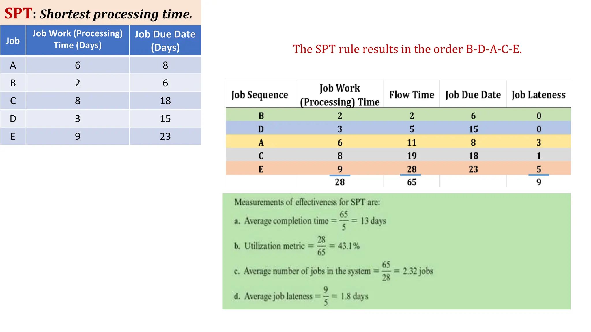
The image below provides another concise example, showing the initial job data, the resulting SPT sequence, and the calculation of key performance metrics.
Test your understanding!
You are given six jobs to schedule on a single machine. Their processing times (in hours) are:
- Job 1: 8
- Job 2: 3
- Job 3: 12
- Job 4: 5
- Job 5: 3
- Job 6: 9
- What is the optimal sequence according to the SPT rule?
- What are the completion times for each job in this sequence?
- What is the minimum total completion time ()?
Show answer
-
Optimal Sequence: First, sort the jobs by their processing times:
- Job 2 (3h), Job 5 (3h), Job 4 (5h), Job 1 (8h), Job 6 (9h), Job 3 (12h).
- Since Job 2 and Job 5 have the same processing time, their relative order can be arbitrary. Let's use the sequence: [2, 5, 4, 1, 6, 3].
-
Completion Times:
-
Total Completion Time:
- hours.
3. Proof of Optimality: The Interchange Argument
As a researcher, it's not enough to know a rule; you must also understand why it is optimal. The standard method to prove the optimality of SPT is the adjacent pairwise interchange argument. The logic is to show that any schedule that is not an SPT schedule can be improved by swapping a pair of adjacent jobs, meaning the non-SPT schedule cannot be optimal.
The SPT rule is a special case of the more general Weighted Shortest Processing Time (WSPT) rule, which is used for the 1 | | Σw_jC_j problem. The proof for WSPT is nearly identical and demonstrates the power of this technique.
The following reading explains this proof clearly.
The following section from 'Chapter 2' formally proves the optimality of the WSPT rule, from which the SPT rule directly follows. This is a classic and very important proof in scheduling theory.
Please read Section 2.4.1 'The WSPT-Rule'. Focus on the 'Proof' section (starting on page 15). Follow the logic: Start with an arbitrary schedule S that violates the rule for an adjacent pair of jobs, i and j. Create a new schedule S* by swapping only i and j. Analyze the change in the total weighted completion time. Notice that only the contributions of jobs i and j change. Show that the new schedule S* has a lower total weighted completion time, thus proving that the original schedule S could not have been optimal. For the SPT case (1 | | ΣCj), you can simply assume all weights w_j are equal to 1.
The core idea of the proof is that for any two adjacent jobs, putting the shorter one first delays the second job by a small amount but brings the first job (and all subsequent jobs) forward by a larger amount, leading to a net reduction in total completion time. This simple, powerful logic ensures the SPT sequence is unbeatable for this objective.
4. Complexity and Final Notes
The SPT rule is computationally efficient. The main work is sorting the n jobs, which can be done in time using an efficient sorting algorithm like mergesort or quicksort. Once sorted, calculating the completion times takes an additional time. Therefore, the 1 | | ΣCj problem is firmly in the class P of polynomial-time solvable problems.
Tie-Breaking: As seen in our exercise, if multiple jobs have the same processing time, their relative order does not affect the total completion time. This means multiple optimal schedules can exist. This freedom can be valuable in practice, as you could use a secondary criterion (like due date) to break ties.
Conclusion
In this lesson, we analyzed our first classic scheduling problem and its optimal solution. We have seen that for the right combination of machine environment and objective, a simple greedy rule can be provably optimal and computationally efficient.
Key Takeaways:
- The problem of minimizing total completion time on a single machine (
1 | | ΣCj) is solved optimally by the Shortest Processing Time (SPT) rule. - The SPT rule is a greedy algorithm: sequence jobs in non-decreasing order of their processing times.
- The optimality of SPT is proven using a powerful pairwise interchange argument, which shows that any non-SPT sequence can be improved.
- Applying the SPT rule is efficient, with a computational complexity of .
Preview of the next lesson:
We will continue our exploration of the single-machine environment, but we will change our performance measure. In the next lesson, we will tackle the problem of minimizing the maximum lateness (1 | | L_max). We will see that this change in objective requires a completely different—but equally elegant—scheduling rule: the Earliest Due Date (EDD) rule.