Hello! Welcome to your next lesson on single-machine scheduling.
In our previous lesson, we saw how the Shortest Processing Time (SPT) rule provides an elegant and provably optimal solution for minimizing total completion time (1 | | ΣCj). We learned the power of a simple greedy algorithm and how to prove its correctness using an interchange argument.
Today, we shift our focus to a different, but equally important, performance objective: meeting deadlines. This lesson addresses the learning outcome: Apply the Earliest Due Date (EDD) rule to minimize maximum lateness on a single machine.
Meeting deadlines is a critical objective in many industrial and service settings. Failing to do so can result in financial penalties, loss of customer goodwill, or disruptions to downstream processes. We will see that this objective also has a simple, optimal greedy solution, reinforcing the theme that understanding the problem structure can lead to highly efficient solutions.
1. Defining Lateness and the Objective Function
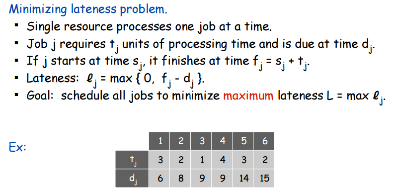
Before we introduce the rule, we need to define our terms precisely. We are still in a single-machine environment where all jobs are available at time zero. However, each job j now has two key parameters:
- A processing time,
- A due date, , which is the time by which the job is expected to be completed.
It's important to distinguish a due date from a deadline. A deadline is typically hard; if a job misses its deadline, the order may be canceled. A due date is softer; missing it is undesirable and may incur costs, but the job is still required. Our focus here is on due dates.
From these parameters, we derive the following performance measures:
- Completion Time (): The time at which job
jfinishes processing. - Lateness (): The difference between a job's completion time and its due date.
Lateness can be positive (the job is late), negative (the job is early), or zero (the job is on time). - Maximum Lateness (): The largest lateness value among all jobs. Our goal is to minimize this value.
In standard notation, this problem is written as 1 | | .
The following image and video provide a clear introduction to these concepts and the problem we aim to solve.
Scheduling to Minimize Maximum Lateness ( Greedy Algorithm ) - Algorithms
To see these definitions in a practical context, watch the beginning of the video 'Scheduling to Minimize Maximum Lateness' from the MisterCode channel. It uses a relatable example of student assignments to explain the concepts.
Watch the segment from 00:30 to 03:23. Focus on how completion time, due date, and lateness are defined and calculated for a given schedule.
2. The Earliest Due Date (EDD) Rule
The optimal solution to the 1 | | Lmax problem is found by applying the Earliest Due Date (EDD) rule, first established by James R. Jackson in 1955. The rule is as intuitive as its name suggests:
To minimize the maximum lateness, process the jobs in non-decreasing order of their due dates.
This greedy strategy prioritizes jobs that are due the soonest, regardless of how long they take to process.
The following segment of the video you just started will walk you through an example, transforming a suboptimal schedule into an optimal one using the EDD rule.
Scheduling to Minimize Maximum Lateness ( Greedy Algorithm ) - Algorithms
Continuing with the 'Scheduling to Minimize Maximum Lateness' video, let's see how applying the EDD rule works in practice and how it improves the schedule.
Watch the segment from 03:23 to 05:20. Observe how sorting the jobs by their due dates creates a new sequence and how this new sequence results in a lower maximum lateness.
Test your understanding!
Consider the set of jobs from the image "The Maximum Lateness: 1||Lmax" (LINK), with the following processing times () and due dates ():

| Job (j) | 1 | 2 | 3 | 4 | 5 |
|---|---|---|---|---|---|
| 6 | 8 | 4 | 7 | 5 | |
| 10 | 12 | 15 | 18 | 22 |
- What is the optimal sequence according to the EDD rule?
- Calculate the completion time () and lateness () for each job in this sequence.
- What is the minimum maximum lateness ()?
Show answer
-
Optimal Sequence: We sort the jobs by their due dates in non-decreasing order:
Job 1 (d=10), Job 2 (d=12), Job 3 (d=15), Job 4 (d=18), Job 5 (d=22).
The sequence is [1, 2, 3, 4, 5]. -
Calculations:
Job (j) 1 6 10 6 6 - 10 = -4 2 8 12 6 + 8 = 14 14 - 12 = 2 3 4 15 14 + 4 = 18 18 - 15 = 3 4 7 18 18 + 7 = 25 25 - 18 = 7 5 5 22 25 + 5 = 30 30 - 22 = 8 -
Maximum Lateness: The lateness values are {-4, 2, 3, 7, 8}.
The maximum lateness is , which occurs for Job 5.
3. Proof of Optimality for the EDD Rule
Given your goal of writing a thesis, understanding the theoretical underpinnings of these classical results is essential. The optimality of the EDD rule can be proven using the same powerful technique we used for the SPT rule: the pairwise interchange argument.
The logic is as follows:
- Assume there is an optimal schedule that is not an EDD schedule.
- If it's not an EDD schedule, it must contain at least one pair of adjacent jobs, say
ifollowed immediately byj, where jobihas a later due date than jobj(). This is called an inversion. - We then show that by swapping jobs
iandj, the maximum lateness of the schedule does not increase (and may even decrease). - By repeatedly swapping such inverted pairs, we can transform any optimal schedule into an EDD schedule without worsening the objective value.
- Therefore, an EDD schedule must be optimal.
The following reading from the textbook by Böhm provides a formal, step-by-step proof of this theorem.
The section 'Maximum lateness' from 'Chapter 2' formally presents Jackson's EDD rule and its proof of optimality. This is a classic result in scheduling theory.
Please read Section 2.5.3, 'Maximum lateness', focusing on the 'Proof of Theorem 2.5.2'. Pay close attention to how the lateness of the two swapped jobs, i and j, changes and why the maximum lateness of the new schedule (S*) is guaranteed to be less than or equal to that of the original schedule (S). This is the heart of the interchange argument.
For a more visual and narrated explanation of a similar proof based on inversions, you can review the final section of the MisterCode video (from 07:20 onwards). Another excellent, in-depth explanation of the exchange argument is provided in the video "Greedy Exchange Arguments" (LINK), which you may find useful for a deeper dive.
4. Complexity and Related Objectives
-
Computational Complexity: Just like the SPT rule, the EDD rule's main computational step is sorting the
njobs. This can be done in time. Thus, the1 | | Lmaxproblem is efficiently solvable and belongs to the complexity class P. -
Maximum Tardiness (): A closely related objective is minimizing maximum tardiness, where . Since the tardiness function is non-decreasing with completion time, the same logic holds: the EDD rule is also optimal for minimizing maximum tardiness (
1 | | Tmax). You can find a brief discussion of this in Section 2.6.1 of the "Chapter 2" text (LINK). -
Lawler's Algorithm: The EDD rule is a special case of a more general procedure called Lawler's Algorithm, which can solve problems of the form
1 | | g_max, whereg_maxis the maximum of some arbitrary non-decreasing cost functions of the completion times. This provides a broader theoretical context for why such greedy, backward-scheduling approaches work.
Conclusion
In this lesson, we have explored another fundamental single-machine scheduling problem. By simply changing the objective from total completion time to maximum lateness, a different priority rule—Earliest Due Date—emerged as optimal.
Key Takeaways:
- The problem of minimizing maximum lateness (
1 | | Lmax) is a key scheduling objective focused on meeting deadlines. - The optimal solution is found by applying the Earliest Due Date (EDD) rule: sequence jobs in non-decreasing order of their due dates.
- The EDD rule's optimality is rigorously proven using a pairwise interchange argument, showing that any schedule with an "inversion" can be improved or at least not worsened.
- The problem is polynomially solvable with a complexity of .
Preview of the next lesson:
So far, we have addressed problems with simple, elegant greedy solutions. However, most real-world scheduling problems, including the FJSP you are researching, do not have such rules. To solve them, we need more powerful and general techniques. In the next lesson, we will make a significant step in that direction by learning how to formulate a single-machine scheduling problem as a Mixed-Integer Linear Program (MILP). This will be our first introduction to mathematical modeling for scheduling, a critical skill for your thesis work.