Welcome to the final module of our course, focusing on the research skills you'll need to complete your thesis. In our last lesson, we laid the groundwork for empirical evaluation by learning how to select appropriate benchmark instances and performance metrics. You now know how to choose the right problems (the "what") and how to measure success (the "how to measure").
Today, we will assemble these pieces into a complete, structured plan. Our learning outcome is to define a formal experimental protocol, including comparison algorithms and parameter tuning strategies. This is one of the most critical sections of a research thesis, as it ensures your work is scientifically rigorous, credible, and reproducible. A well-defined protocol is like the architectural blueprint for your computational experiments; it dictates every step, from setting up the test to analyzing the results.
We will cover three core components:
- Selecting a meaningful set of comparison algorithms to benchmark your proposed method against.
- Implementing a fair and systematic parameter tuning strategy to ensure all algorithms perform at their best.
- Structuring the complete experimental protocol that you can use as a template for your thesis.
Let's begin by outlining what a comprehensive experimental design looks like.
1. The Anatomy of an Experimental Protocol
A robust experimental protocol leaves no room for ambiguity. It tells the reader exactly what you did, how you did it, and why you did it that way. A well-structured protocol in a scheduling paper typically involves several distinct validation steps.
The paper 'Optimization Algorithm for FJSP-AD-LS' by Shen et al. provides an excellent roadmap for a thorough experimental design. Let's look at their methodology to understand the key components.
Please read the section titled 'Step 3: Experimental Design and Analysis'. Pay close attention to the five sub-steps the authors outline. These form a comprehensive framework for validating a new algorithm.
As you saw, the authors broke their experimental plan into five clear stages:
- Test Case Design: Selecting or generating benchmark instances (our previous lesson).
- Parameter Tuning: Optimizing algorithm parameters.
- Ablation Study: Analyzing the contribution of your algorithm's components.
- Model Validation: Comparing against an exact solver on small instances.
- Comparative Experiments: Benchmarking against other state-of-the-art algorithms.
Let's explore these last three validation stages in more detail. They are all centered around a crucial choice: which algorithms will you compare yours against?
2. Choosing Your Opponents: Comparison Algorithms
To prove your algorithm is effective, you must compare it against a thoughtfully chosen set of "opponents." A strong thesis will typically include three types of comparisons.
2.1. Baseline 1: Validation Against Exact Methods
For many NP-hard problems, exact methods like MILP or CP can find the proven optimal solution, but only for small instances before their runtime becomes impractical. Comparing your algorithm to an exact solver (like Gurobi or CPLEX) on small problems serves two purposes:
- It validates your own model and implementation. If your heuristic finds a solution on a small instance that is worse than the proven optimum, that's fine. But if the solver finds no feasible solution while your heuristic does, it might indicate an error in your MILP/CP model formulation.
- It justifies the need for your heuristic. By showing that the exact solver fails to find solutions for larger instances within a reasonable time limit, you demonstrate why heuristics and metaheuristics are necessary for solving industrially-relevant problems.
The paper by Shen et al. performs exactly this kind of validation.
Let's examine how Shen et al. used Gurobi to validate their MILP model and demonstrate the superiority of their proposed metaheuristic (AMGWO) on larger problems.
Please read section '6.4 MILP validation'. Notice how they report the results from the MILP solver (Gurobi) and their AMGWO algorithm in Table 8. Focus on their conclusion: the MILP works for small-scale problems but fails as the scale increases, while AMGWO consistently finds superior results.
2.2. Baseline 2: Comparison with State-of-the-Art (SOTA)
This is the main event of your experimental chapter. To claim your algorithm is a valuable contribution, you must show that it performs favorably against other high-quality algorithms from recent literature that solve the same, or a very similar, problem.
This involves:
- Identifying 2-4 relevant algorithms from your literature review.
- Re-implementing them or, if available, using the authors' original code.
- Running them on the same benchmark instances under the same conditions.
Let's see how Shen et al. compare their AMGWO algorithm against other metaheuristics.
Please read section '6.5 Performance comparison'. Observe how they selected four other recent methods (GA-VNS, EMA, SCEGWO) and compared the results in detail in Tables 7, 8, and 9. Also, look at Figure 19, which compares the convergence curves—another powerful way to visualize performance.
2.3. Baseline 3: The Ablation Study
If your proposed algorithm combines several novel ideas (e.g., a new crossover operator, a local search procedure, and a special initialization), how do you prove that each component contributes positively? The answer is an ablation study.
In an ablation study, you test stripped-down versions of your own algorithm. For example, if your full algorithm is "GA + VNS", you would compare:
- Full Algorithm: GA + VNS
- Ablation 1: GA only (VNS removed)
- Ablation 2: A baseline algorithm (e.g., a simple GA)
If the full algorithm outperforms the ablated versions, you have strong evidence that your specific combination of components is effective.
Shen et al. conduct a textbook ablation study to prove the effectiveness of their improvement strategies. Let's analyze it.
Please read section '6.3 Improvement analysis'. The authors compare three versions: the basic GWO, GWO-I (with one improvement), and the full AMGWO (with both improvements). Look at Figure 17 and their analysis of how each added component improves the median makespan and reduces solution variance.
3. Fair Play: Parameter Tuning Strategies
Metaheuristics are sensitive to their parameter settings (e.g., population size, mutation rate, tabu list length). A common flaw in experimental research is to compare a meticulously tuned new algorithm against poorly tuned SOTA algorithms. This is not a fair or scientific comparison.
A rigorous experimental protocol must include a systematic and transparent parameter tuning phase. Given your background in industrial engineering, you may already be familiar with powerful statistical tools for this, such as Design of Experiments (DOE).
One of the most widely used methods in scheduling research is the Taguchi method.
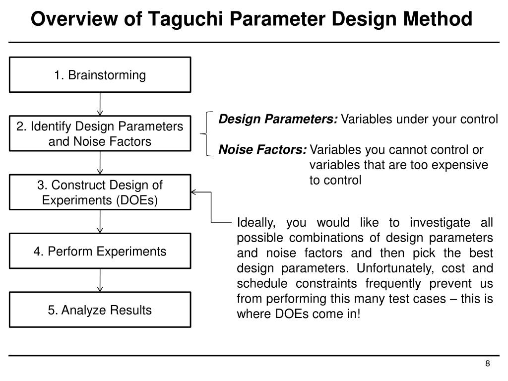
The Taguchi method allows you to explore the parameter space efficiently and identify the most influential parameters and their optimal levels.
Let's see a practical application of this method.
The Shen et al. paper provides an excellent, detailed example of using the Taguchi method to tune the parameters of their AMGWO algorithm. This is a model you can follow directly in your own thesis.
Please carefully study section '6.2 Parameter settings'. Pay attention to: The identification of key parameters to be tuned (ps, pn, pr_max, pt). Table 5, which defines the different 'levels' (values) for each parameter. Table 6, which shows the L16 orthogonal array—the experimental plan that combines different parameter levels. The use of Relative Percent Deviation (RPD) as the response variable to measure performance. Figures 15 and 16, which are used to analyze the results and select the best parameter configuration.
By using and documenting a systematic method like Taguchi, you demonstrate that you have made a good-faith effort to find strong parameter settings, which adds significant credibility to your results.
4. Assembling the Formal Protocol
Now, let's consolidate everything into a single, formal protocol. This is the template you can adapt for your thesis. A complete protocol should clearly state the following:
-
Experimental Objectives:
- What specific questions are your experiments designed to answer?
- Example: "To demonstrate that the proposed hybrid CP-GA algorithm finds higher quality solutions for the FJSP with transport constraints compared to standalone GA and CP models, particularly on large-scale instances."
-
Benchmark Instances:
- Which benchmark libraries will be used? (e.g., Brandimarte, Dauzère-Pérès).
- How will you select instances? (e.g., "A selection of 5 small, 5 medium, and 5 hard instances...").
- If adapting or generating instances, what is the exact procedure? (e.g., "Sequence-dependent setup times were generated from a uniform distribution U[10, 50]...").
-
Comparison Algorithms:
- List the baselines (exact solvers, simple heuristics) and SOTA algorithms you will compare against.
- Justify your choices (e.g., "Algorithm X was chosen as it represents the current SOTA for FJSP with sequence-dependent setups.").
-
Performance Metrics:
- What metrics will be used to evaluate performance? (e.g., RPD from BKS, objective function value, computation time).
-
Parameter Tuning Procedure:
- Describe the method used to tune parameters for your algorithm and the comparison algorithms (e.g., "The Taguchi method with an L16 orthogonal array was employed...").
- Report the final parameter settings used for all algorithms in all experiments.
-
Computational Environment:
- Specify the hardware (CPU, RAM) and software (OS, language, library/solver versions). This is essential for reproducibility and fair time comparisons.
- Example: "All experiments were run on a machine with an Intel Core i7-8700 CPU and 16GB of RAM. The algorithms were implemented in Python 3.9, using Gurobi 10.0.3 as the MILP solver."
-
Execution and Termination:
- How many times will each stochastic algorithm be run on each instance? (e.g., 10 or 30 independent runs).
- What are the termination criteria? (e.g., a maximum computation time limit, a target optimality gap). The paper by Joshi et al. provides a good example of an early termination criterion for a MILP model.
Test your understanding!
You are designing an experiment to test your new metaheuristic, "Hybrid-TS-GA," for the FJSP. In your literature review, you found that a recent algorithm called "FastGA" is considered state-of-the-art. Your algorithm has two key parameters: tabu list size and population size.
Based on today's lesson, outline three essential comparisons you should include in your experimental protocol to make a strong case for your algorithm.
Show answer
A strong experimental protocol would include these three comparisons:
- Comparison with an Exact Solver: Run Hybrid-TS-GA and a Gurobi/CPLEX MILP model on small-scale FJSP instances (e.g., from Brandimarte). This validates your model and demonstrates the need for a metaheuristic on larger instances where the solver fails.
- Comparison with State-of-the-Art: Run Hybrid-TS-GA against "FastGA" on a wide range of medium and large benchmark instances. This is the core comparison to show your algorithm is competitive with or superior to existing methods. You must also describe how you tuned the parameters for both algorithms fairly.
- Ablation Study: Run two simplified versions of your algorithm—"TS only" and "GA only"—against the full "Hybrid-TS-GA". This will provide evidence that the hybrid combination of Tabu Search and a Genetic Algorithm is what provides the performance benefit, rather than just one of the components.
Conclusion
You now have a complete blueprint for designing a rigorous, credible, and defensible computational study for your thesis. A formal experimental protocol is not just a formality; it is the bedrock of your empirical claims.
Key Takeaways:
- A formal protocol consists of defining benchmarks, metrics, comparison algorithms, parameter tuning methods, and the computational environment.
- Compare your algorithm against three key baselines: exact solvers (for validation), state-of-the-art algorithms (for competitiveness), and ablated versions of itself (to prove your ideas work).
- Parameter tuning is not an afterthought. Use a systematic method like the Taguchi design and report your procedure transparently to ensure a fair comparison.
- Document every detail of your protocol to ensure your research is reproducible.
Preview of the Next Lesson:
You have designed the experiment. The next step is to run it and make sense of the data. In our next lesson, we will focus on how to "Interpret and report experimental results following academic research standards." We will cover how to create effective tables and charts, perform basic statistical analysis, and draw meaningful conclusions from your data.