Python Data Structures: Time and Space Complexity

Hello! Welcome to the final lesson of our first module on algorithmic analysis.

In our last lesson, you learned how to define your own custom data structures using Python classes by building a basic LinkedList. This was a big step, as it showed how to create new data types from scratch.

Today, we'll shift our focus back to the powerful data structures that Python provides right out of the box: lists and dictionaries. Our goal is to analyze the time and space efficiency of their common operations. Understanding how these built-in types perform under the hood is one of the most practical skills for a data-focused role. In an interview, choosing the right data structure for a problem—and being able to justify that choice with Big O notation—is a key signal of your expertise.

Why Performance Matters: A Quick Refresher

As a reminder from our earlier lessons on Big O notation, the efficiency of an operation describes how its runtime or memory usage scales as the input size (n) grows.

O(1) (Constant Time): The operation takes the same amount of time regardless of the size of the data structure. This is ideal.
O(n) (Linear Time): The time taken grows in direct proportion to the number of elements. This is acceptable, but can be slow for very large n.
O(log n) (Logarithmic Time): The time taken grows very slowly as the size increases. This is very efficient.

Let's dive in and see how these apply to Python's most-used data structures.

1. The Workhorse: Python `list`

In Python, a list is not a linked list like the one we built. It's actually a dynamic array. This means it stores its elements in a contiguous block of memory, like seats in a single row of a movie theater. This underlying implementation has direct consequences for its performance.

Python for Coding Interviews - Everything you need to Know

To start, let's get a quick overview of list operations. This clip from NeetCode's guide for coding interviews demonstrates several key list methods and mentions the time complexity for one of them.

Watch the segment from 08:28 to 10:11. Pay attention to the operations mentioned: append, pop, insert, and indexing (my_list[0]). Notice the comment about the time complexity of insertion.

As the video hinted, not all list operations are equally fast. Let's break down why.

Time Complexity of List Operations

Accessing an element by index (my_list[i]): O(1)
Since the list's data is in one continuous block of memory, Python can instantly calculate the memory address of any element using its index. It doesn't need to search; it can jump directly there.
Appending to the end (my_list.append(item)): O(1) (Amortized)
Adding an item to the end is usually very fast. Python keeps track of the end of the list and just places the new item there. Occasionally, the list runs out of allocated space and needs to be resized—a process that involves allocating a new, larger block of memory and copying all existing elements over. This resize is an O(n) operation. However, because it happens infrequently, the cost is "amortized" (spread out) over many appends, making the average cost O(1).
Popping from the end (my_list.pop()): O(1)
Removing the last item is also a constant-time operation, as no elements need to be shifted.
Inserting or Deleting at an arbitrary position (my_list.insert(i, item), my_list.pop(i)): O(n)
This is the most important performance characteristic to remember for lists. To understand why it's O(n), let's get a clearer explanation.

Python Data Structures: Lists

This article from Anaconda explains the performance of lists very clearly. It gives a great analogy for why insertion and deletion are slow.

Read the subsection 'List performance characteristics'. The example of removing the first element from a list of 1 million items perfectly illustrates the concept of shifting elements.

As the article explains, if you insert an element at the beginning of a list, every single other element must be shifted one position to the right to make room. Similarly, deleting an element from the beginning requires shifting all subsequent elements to the left to fill the gap. This "shifting" work is proportional to the number of elements being moved, leading to O(n) complexity.

Searching for an element (item in my_list): O(n)
To check if an item exists in a list, Python has to, in the worst case, look at every single element from beginning to end until it finds a match.

Space Complexity of Lists

The space complexity of a list is O(n). This is intuitive: the amount of memory needed is directly proportional to the number of elements you store in it.

2. The Key to Speed: Python `dict` and `set`

Dictionaries (dict) and sets (set) are fundamentally different from lists. They are implemented using a hash table. This structure is optimized for one thing above all else: fast lookups, insertions, and deletions.

How Hash Tables Work (The Simple Version)

Imagine a large filing cabinet with thousands of drawers, each with a unique number.

Hashing: When you want to store a piece of data (e.g., the value 28 associated with the key "alice"), Python doesn't search for an empty spot. Instead, it runs the key ("alice") through a special hash function. This function instantly converts the key into a number, which corresponds to a drawer number.
Storage/Retrieval: Python then goes directly to that drawer to store or retrieve the value.

This process avoids a linear scan. As long as the hash function is good and doesn't send too many different keys to the same drawer (a "collision"), the operation is incredibly fast.

Python Data Structures: Dictionaries and Hashed Tables

The same Anaconda article provides an excellent, non-technical explanation of how dictionaries use hashing to achieve their speed.

Please read the subsection 'How dicts stay fast'. The analogy of using a phone book's tabs instead of reading every page is a great way to think about it.

Time Complexity of Dictionary and Set Operations

Because of this hashing mechanism, the performance of dictionaries is remarkable:

Accessing an item (my_dict[key]): O(1) (Average)
Inserting or Updating an item (my_dict[key] = value): O(1) (Average)
Deleting an item (del my_dict[key]): O(1) (Average)
Checking for a key (key in my_dict): O(1) (Average)

A set is essentially a dictionary that only stores keys (with no associated values). It uses the exact same hash table machinery, so its performance is identical for its core operations: add, remove, and membership testing (item in my_set) are all O(1) on average.

The "average" note is because in the rare case of many hash collisions, performance can degrade to O(n). However, in practice, you can almost always assume O(1) behavior.

Space Complexity of Dictionaries and Sets

The space complexity for both is O(n), where n is the number of key-value pairs (for dicts) or elements (for sets).

3. Comparing `list` vs. `set` for Lookups

The difference between an O(n) list search and an O(1) set search is one of the most important performance trade-offs in Python.

Python Sets Tutorial #1 & Time Complexity (BIG O)

This video by Tech With Tim offers a fantastic explanation of why checking for an element in a set is so much faster than in a list.

Watch the segment from 04:43 to 08:35. It introduces Big O notation in this context and clearly contrasts the for loop required for a list search (O(n)) with the direct lookup in a set (O(1)).

Summary and Practical Application

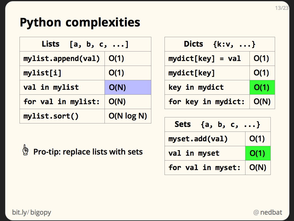
Let's consolidate everything into a clear summary. The following image is a great cheat sheet for the performance of these data structures.

Python Complexities for Lists, Dictionaries, and Sets — A table summarizing the Big O time complexities for common operations on Python lists, dictionaries, and sets. It highlights the key performance differences, especially for membership testing.

Test your understanding! (Interview Scenario)

You are working on a data pipeline. You're given a file containing 10 million transaction IDs. You are also given a separate list of 5,000 "fraudulent" transaction IDs. Your task is to write a script that counts how many of the fraudulent IDs appear in the main transaction log.

You load the 10 million transaction IDs into a Python list. What is the most efficient way to perform the check?

Iterate through your list of 5,000 fraudulent IDs. For each one, use the in operator to check if it's in the 10-million-item list.
First, convert the 10-million-item list into a set. Then, iterate through your list of 5,000 fraudulent IDs, and for each one, use the in operator to check if it's in the newly created set.

Which approach is better and why? Think about the Big O complexity.

Show answer

Approach 2 is vastly more efficient.

Here's the analysis:
Let N be the number of transactions (10 million) and M be the number of fraudulent IDs (5,000).

Approach 1 (Using a list):
- Checking fraud_id in big_list is an O(N) operation.
- You do this M times.
- Total complexity: O(N * M). (Roughly 10,000,000 * 5,000 = 50 billion operations). This would be extremely slow.
Approach 2 (Using a set):
- Step 1: Convert the big list to a set: transaction_set = set(big_list). This takes O(N) time because it has to iterate through all N items once.
- Step 2: Loop through the fraudulent IDs. Checking fraud_id in transaction_set is an O(1) operation. You do this M times. This part takes O(M) time.
- Total complexity: O(N + M). (Roughly 10,000,000 + 5,000 operations). This is significantly faster and will complete in a reasonable amount of time.

This scenario is a classic example of when to use a set for fast membership checking, a very common pattern in data engineering and technical interviews.

Conclusion

Great job today! Understanding the performance characteristics of the tools you use every day is what separates a novice programmer from an effective one.

Key Takeaways:

Lists (Dynamic Arrays): Excel at ordered data and fast access by index (O(1)). Appending/popping from the end is also fast (O(1)). They are slow for insertion, deletion, and searching in the middle (O(n)) because elements may need to be shifted.
Dictionaries & Sets (Hash Tables): Unordered but provide extremely fast insertion, deletion, and lookups (O(1) on average) by leveraging hash functions.
The Main Trade-off: Choose list when order matters and you mostly add to the end. Choose dict or set when you need to do fast lookups and order doesn't matter.

In our next lesson, we will officially start Module 2 by diving deeper into that O(n) search operation. You will implement linear search and analyze its time complexity, kicking off our exploration of fundamental searching and sorting algorithms.

Recommended resources