Understanding the Lee-Carter Model: Structure and Assumptions

Introduction

Welcome to our new module on mortality projection. In the previous lessons, we perfected the art of graduation—creating a smooth, static mortality table that best represents the mortality experience of a population over a specific historical period. However, for many actuarial tasks like pricing life annuities or funding long-term pension schemes, a static snapshot is not enough. We need to account for the fact that mortality rates are not constant; they have been steadily improving for decades.

This lesson introduces the foundational model for this task: the Lee-Carter model. Developed by Ronald Lee and Lawrence Carter in 1992, it was a breakthrough in mortality forecasting, elegantly combining demographic patterns with statistical time series analysis. We will explore the structure of this model, dissect its components, and understand the core assumptions it relies on. Your strong background in statistics and time series will be particularly valuable here, as you'll see familiar concepts applied in a new and powerful way.

Why We Can Model Mortality

Forecasting mortality might seem audacious. How can we predict something as complex as life and death? The feasibility of this task hinges on the remarkable regularity observed in mortality data over long periods and across many countries. To begin, let's hear from one of the creators of the model, Ronald Lee, on why a statistical approach to mortality forecasting is not just possible, but has proven to be quite successful.

Ronald Lee: The Lee-Carter Model - An Update and Some Extensions

This video features Professor Ronald Lee discussing the Lee-Carter model. We will use several clips from this talk.

Please watch the introductory segment from "how is it possible?". As you watch, notice his key point: despite massive changes in the causes of death over the last century, the patterns of mortality decline have remained surprisingly stable and regular. This regularity is what allows for statistical modeling.

The Structure of the Lee-Carter Model

The Lee-Carter model captures this regularity with a surprisingly simple and elegant equation. It models the logarithm of the central death rate at age $x$ in year $t$ , denoted $m_{x, t}$ , as a sum of three components.

The core equation of the model is:

ln (m_{x, t}) = a_{x} + b_{x} k_{t} + ϵ_{x, t}

Let's break this down:

$ln (m_{x, t})$ : The model works with the natural logarithm of the death rate. This is a common statistical technique that helps ensure forecasts of the death rate remain positive and can help stabilize variance and linearize relationships.
$a_{x}$ : This is an age-specific parameter that represents the average log-mortality at age $x$ over the entire period of observation. It captures the general shape of the mortality curve (e.g., high in infancy, dipping in childhood, and then steadily rising through adulthood).
$k_{t}$ : This is a time-specific parameter, often called the "mortality index." It captures the overall level of mortality in year $t$ . Crucially, $k_{t}$ is what drives the model's dynamics. A consistently decreasing $k_{t}$ represents the general trend of mortality improvement over time.
$b_{x}$ : This is another age-specific parameter. It measures the sensitivity of the log-mortality rate at age $x$ to changes in the overall mortality index $k_{t}$ . A high value of $b_{x}$ means that mortality at age $x$ improves rapidly when the general trend $k_{t}$ goes down. A low $b_{x}$ means it improves more slowly.
$ϵ_{x, t}$ : This is the error term, representing random fluctuations or historical details not captured by the main structure of the model.

Let's watch Professor Lee explain this structure himself.

Ronald Lee: The Lee-Carter Model - An Update and Some Extensions

We'll continue with the same video from Bayes Business School.

Now watch the segment from the model explanation. Professor Lee introduces the equation and explains the function of each component. He also points out what the basic model doesn't capture, such as specific shocks (like the 1918 flu pandemic) or cohort-specific factors. This directly addresses the core of today's learning outcome.

As a statistician, you can think of this as a type of factor model. We are decomposing a matrix of log-mortality rates (with ages on one axis and time on the other) into a single dominant factor of time ( $k_{t}$ ) and its age-specific loadings ( $b_{x}$ ), adjusted by a baseline age profile ( $a_{x}$ ).

Visualizing the Lee-Carter Components

The parameters $a_{x}$ , $b_{x}$ , and $k_{t}$ are not just abstract symbols; they are estimated from historical data and have distinct, interpretable shapes. The image below shows a typical plot of these estimated parameters for a male population.

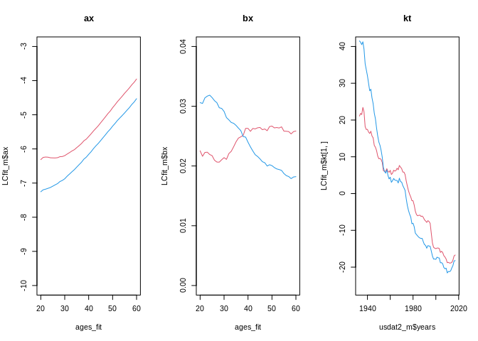
Plots of the estimated Lee-Carter parameters. The left plot shows the age profile of mortality, $a_x$. The middle plot shows the age-specific sensitivity to change, $b_x$. The right plot shows the time series of the mortality index, $k_t$. The red and blue lines typically represent fits to different datasets or different estimation methods.

Let's analyze these plots in light of the model structure:

ax plot (left): This shows the general age-pattern of mortality. As expected, the log-mortality rate increases steadily with age for the adult ages shown (20-60). This represents the average shape of the mortality curve over the entire historical period.
bx plot (middle): This shows how responsive each age is to the general mortality trend. Where the $b_{x}$ curve is higher, mortality rates change more rapidly as $k_{t}$ changes. The plot here shows varied sensitivities across different ages.
kt plot (right): This is the time series of the overall mortality index. The clear and persistent downward trend from 1940 to 2020 is the visual representation of "mortality improvement"—people are living longer. This is the component that we will forecast using time series methods in a future lesson.

Model Assumptions and Identifiability

For the model to work and for its parameters to be meaningful, we must make several key assumptions. It's crucial to understand these, as they are also the model's main limitations.

Time-Invariant Age Effects: The model assumes the main age pattern ( $a_{x}$ ) and the age-specific sensitivities ( $b_{x}$ ) are constant over time. All the dynamics of mortality change are captured by the single index $k_{t}$ . This is a strong assumption; for example, in reality, the pace of mortality improvement at older ages might accelerate over time, which would imply a changing $b_{x}$ .
One-Factor Model: It assumes a single factor ( $k_{t}$ ) drives mortality change at all ages. This implies a high degree of correlation in mortality improvements across the age spectrum. It struggles to model periods where, for instance, young adult mortality worsened (e.g., due to the AIDS epidemic) while older-age mortality continued to improve.
No Cohort Effects: The model is a "period" model, meaning it focuses on death rates in a given calendar year. It does not explicitly account for "cohort" effects—the unique mortality experience of a group of people born in the same year as they age.
Error Structure: The error terms $ϵ_{x, t}$ are assumed to have a mean of zero and constant variance, and to be uncorrelated across time and age.

To formalize our understanding, let's consult a more technical description of the model and its assumptions.

[PDF] the lee-carter model under the condition of variables age ... - SOA.org

This research paper from the Society of Actuaries provides a concise, formal definition of the model.

Please read section 1.1 Lee-Carter model. Focus first on the equation. Note the use of Greek letters (\alpha, \beta, \kappa) which is common in the literature, but the structure is identical to what we've seen. Next, pay close attention to the paragraph starting with "The LC model assumes..." in section 1.2. This explicitly states the key assumption of time-invariance we just discussed.

Identifiability Constraints

A final, crucial point relates to a concept you'll be familiar with from statistical modeling: identifiability. As presented, the equation $ln (m_{x, t}) = a_{x} + b_{x} k_{t}$ does not have a unique solution for its parameters. For example, if we replace $b_{x}$ with $c \cdot b_{x}$ and $k_{t}$ with $k_{t} / c$ , the product $b_{x} k_{t}$ remains unchanged.

To ensure a unique and interpretable set of parameters, we must impose constraints. The standard constraints are:

t \sum k_{t} = 0 and x \sum b_{x} = 1

These constraints give the parameters a clear interpretation:

With $\sum_{t} k_{t} = 0$ , the parameter $a_{x}$ becomes the simple average of $ln (m_{x, t})$ over time.
With $\sum_{x} b_{x} = 1$ , the $b_{x}$ values can be seen as distributing the impact of the overall trend $k_{t}$ across the different ages.

The paper you just read also mentions these constraints right after presenting the model equation.

Conclusion

In this lesson, we have taken our first step from static analysis to dynamic forecasting. We've dissected the Lee-Carter model, the workhorse of mortality projection.

Key Takeaways:

Model Purpose: The Lee-Carter model aims to describe and forecast the entire surface of age-specific death rates over time.
Core Structure: It decomposes the logarithm of death rates into three components:
- $a_{x}$ : An average age profile.
- $k_{t}$ : A single time-series index representing the overall level of mortality.
- $b_{x}$ : A measure of how quickly each age's mortality responds to the general trend.
Key Assumptions: The model's primary assumptions are that the age-specific components ( $a_{x}$ and $b_{x}$ ) are constant over time and that a single factor ( $k_{t}$ ) drives all mortality change. It also does not explicitly model cohort effects.
Identifiability: Constraints such as $\sum_{t} k_{t} = 0$ and $\sum_{x} b_{x} = 1$ are required to ensure a unique solution for the parameters.

Preview of the Next Lesson

We have now described the model's structure and what its components represent. The next logical question is: how do we find the values of $a_{x}$ , $b_{x}$ , and $k_{t}$ from a set of historical data? In the next lesson, we will answer this by learning how to estimate the Lee-Carter model parameters using a powerful matrix factorization technique called Singular Value Decomposition (SVD).

Recommended resources