Moments of Aggregate Claims in the Collective Risk Model

Introduction

In our previous lesson, we focused on the mechanics of reinsurance, calculating how specific claim amounts are divided between an insurer and a reinsurer. We now shift our perspective from individual transactions to the statistical nature of the entire portfolio of claims. This lesson introduces the collective risk model, a cornerstone of modern actuarial science for modeling an insurer's total claim liability.

Our goal is to understand and quantify the uncertainty inherent in the aggregate claims of a portfolio over a given period. Instead of looking at a single loss amount, we will treat the total loss as a random variable and calculate its key statistical properties—specifically, its mean and variance. Your background in probability theory will be especially useful here, as we will be working with the moments of a random sum of random variables. By the end of this lesson, you will be able to state and apply the standard formulas for the expected value and variance of aggregate claims, a skill essential for pricing, reserving, and risk management.

The Collective Risk Model

In actuarial science, the total amount of claims an insurer faces in a period (e.g., a year) is uncertain in two distinct ways:

We don't know how many claims will occur.
For each claim that does occur, we don't know how large it will be.

The collective risk model captures this dual uncertainty. We define the aggregate loss, $S$ , as the sum of a random number of individual claim amounts:

S = X_{1} + X_{2} + \dots + X_{N}

Where:

$N$ is a random variable representing the number of claims in the period (the frequency).
$X_{i}$ is a random variable representing the amount of the i-th claim (the severity).

We make a few standard assumptions:

The individual claim severities, ${X_{i}}$ , are independent and identically distributed (i.i.d.).
The claim frequency, $N$ , is independent of the claim severities, ${X_{i}}$ .

The following video provides an excellent introduction to this concept, using the example of customer spending on Amazon to illustrate the two sources of randomness.

compound poisson

This video from Gareth Tribello introduces the idea of a compound process, which is the name for this type of model when the frequency follows a Poisson distribution.

Please watch the introductory segment from the beginning. Focus on how the model separates the randomness of when purchases happen (frequency) from the randomness of how much is spent (severity).

Moments of Aggregate Claims: The General Formulas

To analyze the aggregate loss $S$ , we are primarily interested in its first two moments: the mean ( $E [S]$ ) and the variance ( $V a r (S)$ ). These can be calculated from the moments of the frequency ( $N$ ) and severity ( $X$ ) distributions.

The derivations rely on the laws of iterated expectation and total variance, which you may have encountered in your statistics studies. We will focus on the resulting formulas and their application.

The primary formulas for the collective risk model are presented clearly in the following textbook excerpt.

Chapter 5 Aggregate Loss Models | Loss Data Analytics

This section from Loss Data Analytics derives and states the general formulas for the mean and variance of aggregate losses under the collective risk model.

Please read the section 5.3.1 Moments and Distribution. Begin at the start of the section and read up to, but not including, the first example. Pay close attention to the two main results presented in the blue boxes: the formulas for the mean and the variance of the aggregate loss S_N.

As you've just read, the formulas are:

Mean of Aggregate Loss:
$E [S] = E [N] \cdot E [X]$
This is highly intuitive: the expected total loss is simply the expected number of claims multiplied by the average size of each claim.
Variance of Aggregate Loss:
$V a r (S) = E [N] \cdot V a r (X) + V a r (N) \cdot (E [X])^{2}$
This formula is less obvious but just as important. It shows that the total variance comes from two sources:
- The variance of the severities: The term $E [N] \cdot V a r (X)$ represents the variance we'd expect if the number of claims was fixed at its mean.
- The variance of the frequency: The term $V a r (N) \cdot (E [X])^{2}$ represents the additional variance introduced because the number of claims itself is random.

Let's apply these formulas to a concrete example.

Chapter 5 Aggregate Loss Models | Loss Data Analytics

This example from Loss Data Analytics applies the general formulas to a scenario where the claim frequency is not Poisson-distributed.

Please study Example 5.3.2. Follow the solution step-by-step to see how the moments of N and X are first calculated and then combined using the general formulas for E[S_N] and Var(S_N).

Let's summarize the calculation from that example:

Frequency Moments:
- $E [N] = 1 (0.8) + 2 (0.2) = 1.2$
- $E [N^{2}] = 1^{2} (0.8) + 2^{2} (0.2) = 1.6$
- $V a r (N) = E [N^{2}] - (E [N])^{2} = 1.6 - 1. 2^{2} = 0.16$
Severity Moments:
- $E [X] = 0 (0.2) + 100 (0.7) + 1000 (0.1) = 170$
- $V a r (X)$ is calculated as $78, 100$ .
Aggregate Moments:
- $E [S] = E [N] E [X] = 1.2 \times 170 = 204$
- $V a r (S) = E [N] V a r (X) + V a r (N) (E [X])^{2} = 1.2 (78, 100) + 0.16 (17 0^{2}) = 98, 344$

The Compound Poisson Process

A very common and important special case of the collective risk model is when the claim frequency $N$ follows a Poisson distribution. Let $N \sim Poisson (λ)$ . In this case, the aggregate loss $S$ is said to follow a compound Poisson distribution.

The key property of the Poisson distribution that simplifies our work is that its mean and variance are equal:

E [N] = V a r (N) = λ

Substituting this into our general variance formula gives a much simpler result:

V a r (S) = E [N] \cdot V a r (X) + V a r (N) \cdot (E [X])^{2} = λ \cdot V a r (X) + λ \cdot (E [X])^{2} = λ \cdot (V a r (X) + (E [X])^{2})

Recalling the relationship $V a r (X) = E [X^{2}] - (E [X])^{2}$ , we see that $V a r (X) + (E [X])^{2} = E [X^{2}]$ .

This leads to the specialized formulas for the Compound Poisson Process:

Mean: $E [S] = λ \cdot E [X]$
Variance: $V a r (S) = λ \cdot E [X^{2}]$

These simplified formulas are frequently tested. Notice that the variance now depends on the second moment of the severity distribution ( $E [X^{2}]$ ), not its variance.

Let's see this in action with another example from the textbook.

Chapter 5 Aggregate Loss Models | Loss Data Analytics

This example demonstrates the application of the simplified formulas for a compound Poisson process.

Now, please read Example 5.3.1. The solution shows two ways to calculate the variance. The first method uses the simplified formula Var(S_N) = \lambda E(X^2). The second method uses the general formula to show it gives the same result.

As the example shows, with $λ = 12$ and $E [X^{2}] = 10/3$ , the calculation is direct:

V a r (S) = λ \cdot E [X^{2}] = 12 \times \frac{10}{3} = 40

This is much quicker than calculating $E [X]$ and $V a r (X)$ separately and using the general formula, though it's reassuring that both methods yield the same answer.

The Shape of the Aggregate Loss Distribution

While we've focused on calculating the first two moments, it's helpful to visualize what the distribution of the aggregate loss $S$ looks like. For portfolios where the expected number of claims $λ$ is large, the Central Limit Theorem suggests that the distribution of $S$ will be approximately normal.

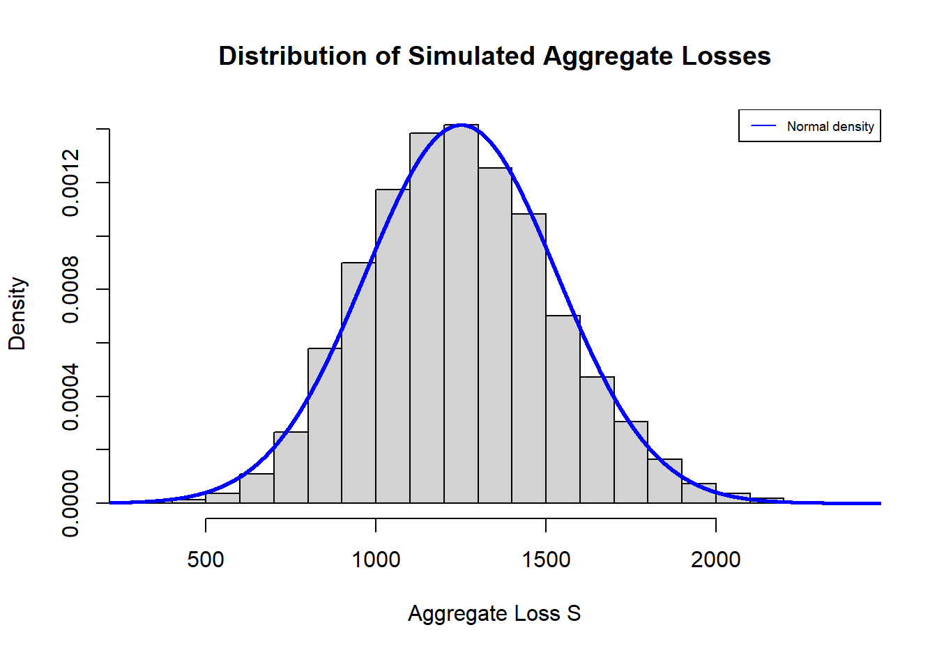
This histogram shows the distribution of simulated aggregate losses from a portfolio. The overlaid blue curve is a Normal distribution with the same mean and variance. As you can see, the Normal distribution provides a reasonable approximation.

The mean and variance we have just learned to calculate, $E [S]$ and $V a r (S)$ , would serve as the parameters for this Normal approximation, $S \cdot \sim N (E [S], V a r (S))$ .

The tendency toward a bell shape is also driven by the frequency distribution itself. As the parameter $λ$ of a Poisson distribution increases, its shape becomes more symmetric and bell-like, resembling a Normal distribution.

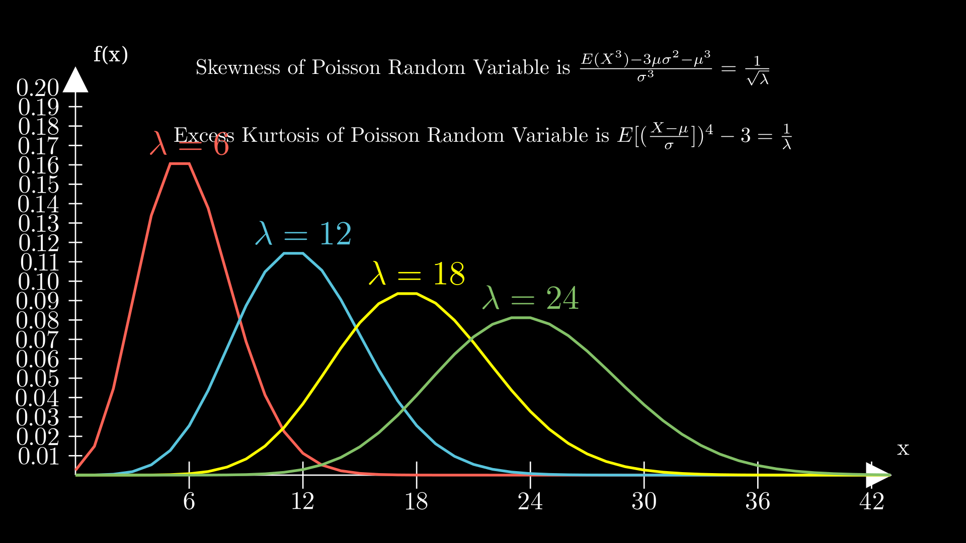
This graph shows how the shape of the Poisson probability mass function changes as its mean, $\lambda$, increases. For larger $\lambda$, the distribution becomes more symmetric and less skewed.

This connection is valuable because it means the moments we calculate are not just abstract numbers; they describe the center and spread of a tangible, often bell-shaped, distribution that represents the insurer's total risk.

Conclusion

In this lesson, we have established the framework for modeling aggregate claims and derived the essential formulas for its mean and variance. These calculations are fundamental to actuarial work, forming the basis for many other tasks.

Key Takeaways:

The collective risk model represents total claims $S = \sum_{i = 1}^{N} X_{i}$ by combining a frequency distribution ( $N$ ) and a severity distribution ( $X$ ).
The general formulas for the moments of aggregate claims are:
- $E [S] = E [N] \cdot E [X]$
- $V a r (S) = E [N] \cdot V a r (X) + V a r (N) \cdot (E [X])^{2}$
For the important special case of a Compound Poisson Process, where $N \sim Poisson (λ)$ , the formulas simplify to:
- $E [S] = λ \cdot E [X]$
- $V a r (S) = λ \cdot E [X^{2}]$

Preview of the Next Lesson

We have now characterized the aggregate claims distribution by its first two moments. However, for a deeper understanding of an insurer's solvency, we need to consider the entire distribution, particularly its tail. In the next lesson, we will introduce the concept of the adjustment coefficient. This parameter, derived from the moment generating function of the aggregate claims distribution, is a key ingredient in estimating the ultimate probability of ruin for an insurer. This will be our first step into the formal study of Ruin Theory.

Recommended resources

Introduction

The Collective Risk Model

Moments of Aggregate Claims: The General Formulas

The Compound Poisson Process

The Shape of the Aggregate Loss Distribution

Conclusion

Preview of the Next Lesson