Survival Analysis Functions and Their Applications

The Four Pillars of Survival Analysis

Any continuous, non-negative random variable $T$, representing a "lifetime," can be described in four equivalent ways. You are likely familiar with the first two from your statistics background, but the latter two are central to survival analysis and actuarial science.

To begin, the following video provides an excellent high-level introduction to these four functions and how they relate to one another in a simple, intuitive example.

Now, let's formalize these concepts. We will draw our definitions from the "Probability Models in Survival Analysis" text, which provides the precise mathematical language used in the field.

Let's summarize the key functions and their interpretations:

• Survivor Function, $S(t)$: $S(t)=P(T\ge t)$. This is the probability that the event (e.g., death, failure) has not occurred by time $t$. In actuarial science, this is often written as ${}_t{p}_x$ for a life aged $x$. It is a non-increasing function starting at $S(0)=1$ and approaching 0 as $t\to \infty$.

• Probability Density Function (PDF), $f(t)$: For a small $\Delta t$, $f(t)\Delta t\approx P(t\le T\le t+\Delta t)$. This represents the unconditional probability density of failure at time $t$. It is simply the negative derivative of the survivor function: $f(t)=-S^{\prime }(t)$.

• Hazard Function, $h(t)$: Also known as the force of mortality (${\mu }_{x+t}$) or failure rate. For a small $\Delta t$, $h(t)\Delta t\approx P(t\le T\le t+\Delta t\mid T\ge t)$. This represents the instantaneous rate of failure at time $t$, conditional on having survived up to time $t$. This conditioning is the crucial difference between the hazard and the PDF.

• Cumulative Hazard Function, $H(t)$: $H(t)={\int }_0^{t}h(\tau )d\tau$. This represents the total accumulated risk or the "amount" of hazard experienced from time 0 up to time $t$.

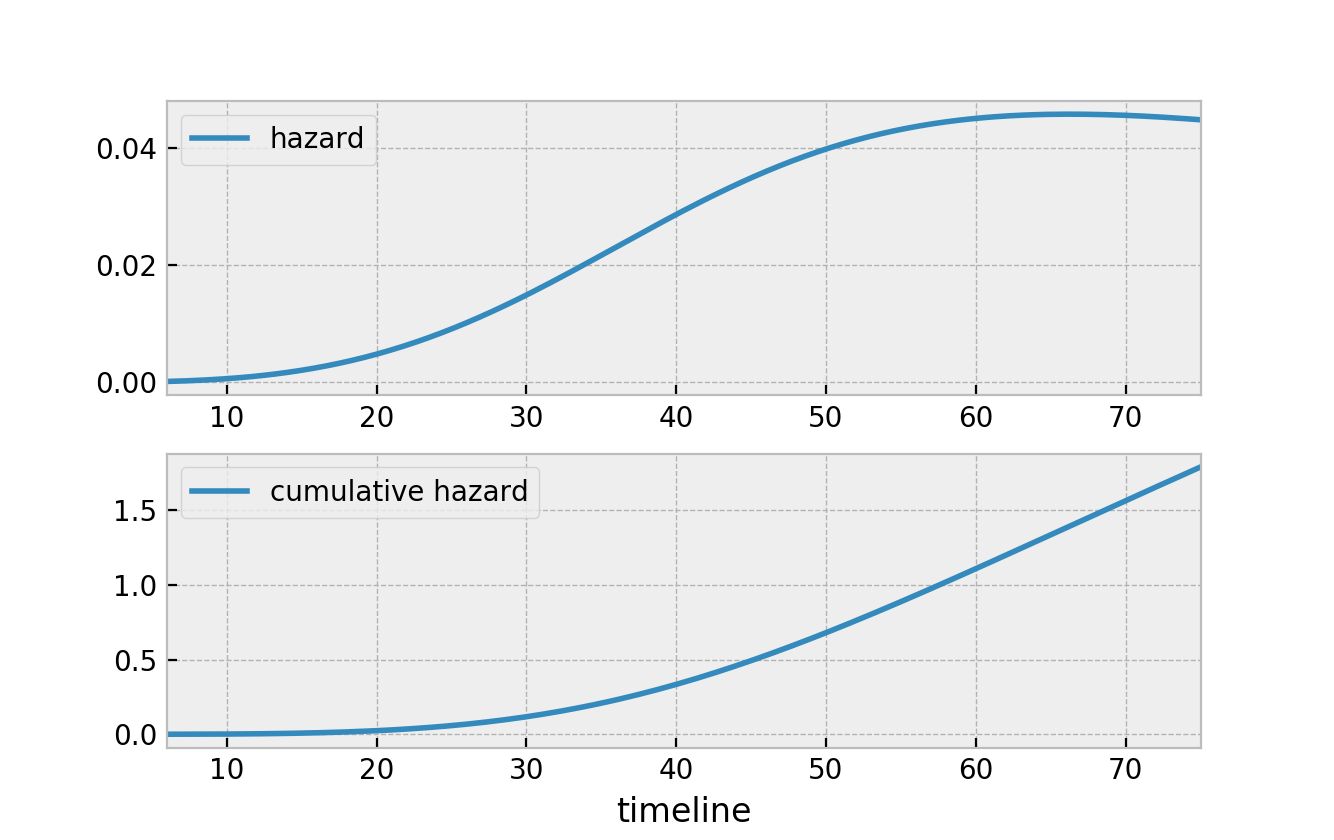
The plot below shows a typical shape for a hazard function and its corresponding cumulative hazard. Notice that as the hazard $h(t)$ increases, the slope of the cumulative hazard $H(t)$ becomes steeper.

The Web of Relationships

These four functions are not independent; they are intrinsically linked through a web of calculus and algebraic relationships. Mastering these conversions is the key to this lesson's objective.

A crucial insight comes from relating the hazard function back to the survivor function. The video below provides a clear, step-by-step derivation.

This derivation reveals the most fundamental relationship in survival analysis:

This single equation allows you to move between the world of survival probabilities and the world of accumulated risk.

All the relationships are summarized in the "from-to matrix" from the Leemis textbook. This table is your primary tool for solving problems.

Let's highlight the most important formulas from this table, which you will use constantly:

Worked Example 1: From Hazard to Everything Else

Let's apply these formulas. Suppose a lifetime $T$ has a linearly increasing hazard function given by $h(t)=0.02t$ for $t\ge 0$. Find the other three functions.

1. Find the Cumulative Hazard Function $H(t)$:
   We integrate the hazard function from 0 to $t$:

   $$H(t)={\int }_0^{t}h(\tau )d\tau ={\int }_0^{t}0.02\tau d\tau ={\left[0.01{\tau }^2\right]}_0^t=0.01t^2$$

2. Find the Survivor Function $S(t)$:
   We use the fundamental relationship $S(t)=e^{-H(t)}$:

   $$S(t)=e^{-0.01t^2}$$

3. Find the Probability Density Function $f(t)$:
   We can use the formula $f(t)=h(t)S(t)$:

   $$f(t)=(0.02t)(e^{-0.01t^2})=0.02t{e}^{-0.01t^2}$$

   Alternatively, we could have differentiated $S(t)$: $f(t)=-S^{\prime }(t)=-(-0.02t\cdot e^{-0.01t^2})=0.02t{e}^{-0.01t^2}$. Both paths lead to the same result.

This distribution is a specific case of the Weibull distribution (with $\kappa =2$), which we will study formally in a later lesson.

Worked Example 2: Application with Conditional Probabilities

Now, let's tackle a problem that uses conditional probabilities, which are common in actuarial work. The following problem is adapted from Example 4.4 in the Leemis text.

Problem: The lifetime of a component, in hours, follows a Weibull distribution with survivor function $S(t)=e^{-(0.0014t{)}^{1.28}}$.
(a) Find the probability that a new component will operate for at least 400 hours.
(b) Find the probability that a component that has already operated for 200 hours will operate for another 400 hours (i.e., until at least 600 hours).

Solution:

(a) Probability a new component survives 400 hours:
This is a direct calculation from the survivor function $S(t)$.

(b) Conditional survival probability:
We need to find $P(T\ge 600\mid T\ge 200)$. Using the definition of conditional probability:

First, we calculate the individual survival probabilities:

Now, we find the ratio:

So, there is a 55.17% chance that a component that has survived for 200 hours will last for another 400 hours. This is lower than the 61.99% probability for a new component because this distribution has an increasing hazard rate (since $\kappa =1.28>1$), meaning the component "wears out" over time.

Practice on an Exam-Style Question

Let's apply these relationships to a question format you might see on the exam. This problem requires you to work backwards from a confidence interval for $H(t)$ to find an interval for $S(t)$.

Problem: A survival study gave (0.283, 1.267) as the symmetric linear 95% confidence interval for $H(5)$. Using the delta method, calculate the symmetric linear 95% confidence interval for $S(5)$.

Solution Strategy:

1. Find the point estimate $\hat{H}(5)$ and the standard error of the estimate, $\text{se}(\hat{H}(5))$, from the given interval.
2. Calculate the point estimate $\hat{S}(5)$ using the relationship $S(t)=e^{-H(t)}$.
3. Use the delta method to find the approximate variance (and standard error) of $\hat{S}(5)$.
4. Construct the 95% confidence interval for $S(5)$.

Step-by-step Calculation:

1. Find $\hat{H}(5)$ and $\text{se}(\hat{H}(5))$:
   A symmetric interval is of the form $\text{estimate}\pm 1.96\times \text{standard error}$.
   The estimate $\hat{H}(5)$ is the midpoint of the interval:

   $$\hat{H}(5)=\frac{0.283+1.267}{2}=0.775$$

   The margin of error is $1.96\times \text{se}(\hat{H}(5))$.

   $$1.96\times \text{se}(\hat{H}(5))=\frac{1.267-0.283}{2}=0.492$$ $$\text{se}(\hat{H}(5))=\frac{0.492}{1.96}\approx 0.251$$

2. Find $\hat{S}(5)$:

   $$\hat{S}(5)=e^{-\hat{H}(5)}=e^{-0.775}\approx 0.4607$$

3. Apply the Delta Method:
   The delta method gives the variance of a function of a random variable. If $g(H)=S=e^{-H}$, then $\text{Var}(\hat{S})\approx [g^{\prime }(\hat{H}){]}^2\text{Var}(\hat{H})$.
   The derivative is $g^{\prime }(H)=-e^{-H}$.

   $$\text{Var}(\hat{S}(5))\approx (-e^{-\hat{H}(5)}{)}^2\times \text{Var}(\hat{H}(5))=(e^{-0.775}{)}^2\times (0.251{)}^2$$ $$\text{Var}(\hat{S}(5))\approx (0.4607{)}^2\times (0.251{)}^2\approx 0.2122\times 0.0630\approx 0.01337$$

   The standard error is the square root:

   $$\text{se}(\hat{S}(5))=\sqrt{0.01337}\approx 0.1156$$

4. Construct the CI for $S(5)$:

   $$\hat{S}(5)\pm 1.96\times \text{se}(\hat{S}(5))=0.4607\pm 1.96\times 0.1156=0.4607\pm 0.2266$$

   This gives the interval $(0.2341,0.6873)$. This corresponds to choice (A) (0.23, 0.69).

Conclusion

In this lesson, we have formally defined the four key functions of survival analysis and, most importantly, established the critical relationships that allow us to move between them. These conversions are not just theoretical exercises; they are the practical tools you will use to solve a wide range of problems in survival modeling.

Key Takeaways:

• A lifetime distribution can be fully specified by its survivor function $S(t)$, PDF $f(t)$, hazard function $h(t)$, or cumulative hazard function $H(t)$.
• The hazard function $h(t)$, or force of mortality ${\mu }_t$, represents the instantaneous risk of failure at time $t$, conditional on survival to that time.
• The fundamental relationships $S(t)=e^{-H(t)}$ and $H(t)=-\ln (S(t))$ are the bridge between survival probability and accumulated risk.
• The "from-to matrix" provides a comprehensive toolkit for deriving any one representation from another, which is a key problem-solving skill.

In our next lesson, we will put the survivor function to immediate use. We will learn how to calculate two of the most important summary measures in actuarial science: the complete and curtate expected future lifetimes, along with their variances.