Vector Database Setup for Document Embeddings

The Core Problem: Searching in High-Dimensional Space

Searching for the "nearest" vectors in a high-dimensional space is a non-trivial problem. The primary challenge lies in the trade-off between search speed and accuracy.

• Exact Nearest Neighbor (k-NN) Search: This method guarantees finding the absolute closest k vectors to your query. It does this by calculating the distance between the query vector and every single vector in the database. While 100% accurate, its computational complexity (linear with the number of vectors) makes it too slow for most real-world applications with large datasets.

• Approximate Nearest Neighbor (ANN) Search: This is the enabling technology behind modern vector search. ANN algorithms trade a small, often negligible, amount of accuracy for a massive gain in search speed—often orders of magnitude faster. The core idea is to intelligently partition the vector space or build a navigational structure so you don't have to search everywhere. For RAG, finding "very good" matches is almost always sufficient and far more practical than finding the "perfect" matches.

To implement ANN search, vector databases use sophisticated indexing structures.

As the article explains, HNSW and IVF are two of the most dominant indexing strategies.

This image visually contrasts the two main ANN indexing algorithms. HNSW (left) uses a multi-layered graph to navigate efficiently from a coarse to a fine level. IVF (right) works by first clustering the data and then restricting the search to the most promising cluster(s) around a query.

Now, let's see how these concepts are implemented in practice.

Practical Implementation 1: FAISS (The High-Performance Engine)

FAISS (Facebook AI Similarity Search) is a low-level, open-source library from Meta AI. It's not a full-fledged database but a highly optimized C++ engine with Python bindings, designed for raw performance and memory efficiency. For an engineer, thinking of FAISS as the "BLAS/LAPACK of vector search" is a fitting analogy.

We'll explore three fundamental FAISS index types that map directly to the concepts we've discussed.

Key Steps with FAISS

As you saw in the video, the typical workflow with FAISS is:

1. Prepare Data: Generate your document embeddings (e.g., as a NumPy array).
2. Instantiate Index: Choose and initialize an index type, providing the vector dimension (d).
   • faiss.IndexFlatL2(d): Brute-force k-NN. No training needed.
   • faiss.IndexIVFFlat(quantizer, d, nlist): Inverted File index. Requires a quantizer index (usually an IndexFlatL2) and the number of clusters (nlist).
   • faiss.IndexIVFPQ(...): Inverted File with Product Quantization. The fastest option, requiring more configuration.
3. Train Index (if needed): Indexes like IVF and IVFPQ must be trained on your data (or a representative sample) to learn the cluster centroids.

   if not index.is_trained:
       index.train(embeddings)
   

4. Add Vectors: Populate the trained index with your embeddings.

   index.add(embeddings)
   

5. Search: Use the index.search() method with your query vector(s) to get the distances and indices of the top-k results.

FAISS gives you fine-grained control but requires you to manage the index's lifecycle, including saving it to disk and loading it back.

Practical Implementation 2: ChromaDB (The Developer-Friendly Database)

Where FAISS is a low-level engine, ChromaDB is a higher-level, open-source, "AI-native" vector database. It's built for ease of use and rapid application development. Chroma manages not only the vectors but also the associated documents and metadata, and it typically uses an efficient ANN index like HNSW under the hood without requiring manual training from the user.

Key Steps with ChromaDB

Chroma's workflow is more declarative and integrated.

The typical workflow is:

1. Install and Get Client:

   import chromadb
   client = chromadb.Client() # Or chromadb.PersistentClient(path="/path/to/db") for on-disk storage
   

2. Create or Get Collection: A collection is like a table that will store your documents, embeddings, and metadata.

   collection = client.get_or_create_collection(name="my_knowledge_base")
   

3. Add Documents: You can add documents directly, and if you provide an embedding function, Chroma will handle embedding generation. For more control, we can provide our pre-generated embeddings.

   collection.add(
       embeddings=embeddings, # Your NumPy array of embeddings
       documents=chunk_texts,  # List of original text chunks
       metadatas=[{"source": "doc1.pdf"}, ...], # Optional metadata
       ids=[f"chunk_{i}" for i in range(len(chunk_texts))] # Unique IDs for each chunk
   )
   

4. Query: Search the collection using text queries. Chroma will embed the query using the same process and perform an ANN search.

   results = collection.query(
       query_texts=["What is the capital of France?"],
       n_results=5 
   )
   # results['documents'] will contain the retrieved text chunks
   

Synthesis: Choosing Your Vector Store and Index

As a top-tier engineer, knowing how to use these tools is only half the battle. Knowing when and why to choose one over the other is what sets you apart.

• FAISS vs. ChromaDB:

  • Use FAISS when you need a bare-metal, high-performance library to integrate into a larger system and are comfortable managing the index lifecycle yourself. It's ideal for performance-critical backend services where you want to minimize overhead.
  • Use ChromaDB (or similar like PGVector, Weaviate, Pinecone) when you want a full-featured database that simplifies development. It's better for building end-to-end applications, rapid prototyping, and when you value developer experience and integrated metadata management.

• Anchor Resource: Choosing an Index Type
  The choice of the underlying ANN algorithm (Flat, IVF, HNSW) is a critical engineering decision based on your dataset size, memory constraints, update frequency, and accuracy requirements.

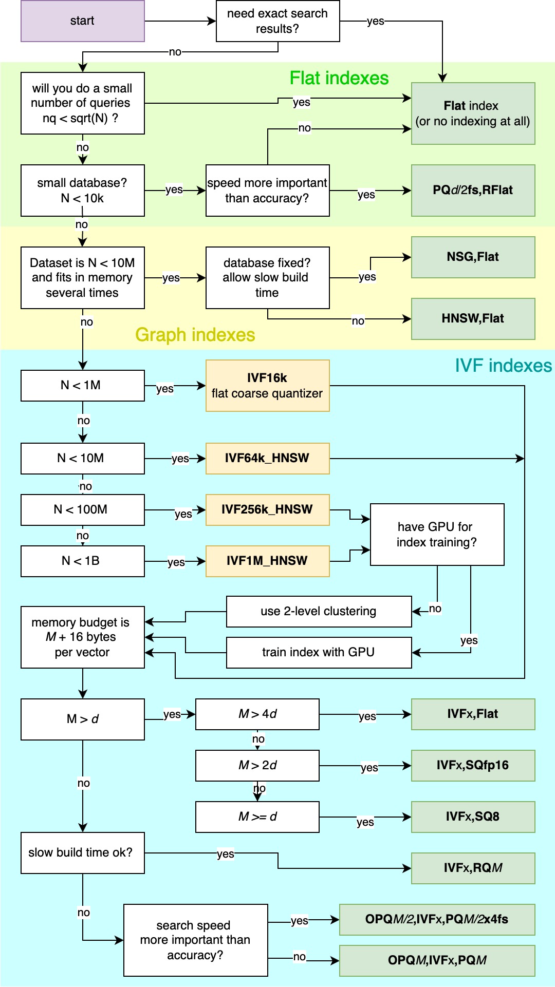
*This flowchart is an excellent mental model for deciding which index type to use. For many modern RAG applications starting with an HNSW-based index (the default in Chroma and an option in FAISS) is a strong baseline due to its excellent performance and the fact that it doesn't require retraining as data is added.*

Conclusion

You have now bridged the gap between having embeddings and having a searchable knowledge base. You've established the foundation of the "Retrieval" in RAG.

Key Takeaways:

• ANN is Key: Approximate Nearest Neighbor (ANN) search is the core technology that makes fast vector retrieval possible by trading a little accuracy for a lot of speed.
• Indexing Strategies Matter: Algorithms like IVF (clustering-based) and HNSW (graph-based) offer different trade-offs in terms of speed, memory, accuracy, and ease of maintenance.
• Tools for the Job: You now have two tools in your arsenal: FAISS, a high-performance library for when you need raw power and control, and ChromaDB, a developer-friendly database for building applications quickly.
• Engineering Decisions: Choosing the right vector store and index type is a critical design decision that depends on your specific application's constraints (dataset size, update frequency, latency requirements, and memory budget).

What's Next?

We have successfully built and populated an indexed vector database. The offline part of our RAG pipeline—chunking, embedding, and indexing—is now complete. The next step is to operationalize the online retrieval process.

In the next lesson, we will focus on implementing the semantic search function itself. You will write the code that takes a user query, embeds it, queries the vector database we've just set up, and retrieves the most relevant document chunks, preparing them to be fed into a large language model.