Introduction
In our last lesson, we compared the leading inference serving frameworks—vLLM, TensorRT-LLM, and TGI—and established a mental model for choosing the right one based on trade-offs between performance, ease of use, and ecosystem support. A recurring theme in that discussion, especially when aiming for maximum performance and cost-efficiency, was quantization.
Today, we will dive deep into this critical optimization technique. As an applied AI engineer, mastering quantization is non-negotiable. It's the key that unlocks the ability to run massive models on smaller, more affordable hardware, drastically reduce inference latency, and ultimately make your LLM applications economically viable.
Our learning outcome is to explain model quantization trade-offs and implement a post-training quantization technique (e.g., GPTQ, AWQ). We will start with the fundamental principles, explore the landscape of modern quantization methods, and then walk through a practical implementation.
The "What" and "Why" of Quantization
At its core, quantization is the process of reducing the numerical precision of a model's weights and, sometimes, its activations. Most models are trained using 32-bit floating-point numbers (FP32), which offer a wide range and high precision. Quantization converts these numbers into lower-precision formats like FP16, BF16, or even 8-bit/4-bit integers (INT8/INT4).
To understand this concept intuitively, let's watch a short, clear explanation.
Which Quantization Method is Right for You? (GPTQ vs. GGUF vs. AWQ)
This clip from Maarten Grootendorst's video provides an excellent visual introduction to quantization. It explains how reducing the number of bits used to represent a value affects its precision.
Watch from 03:18 to 06:24. Focus on the core idea: representing the same information with fewer bits, and the inherent trade-off this creates.
As the video illustrates, this reduction comes with a fundamental trade-off.
The Core Trade-offs of Quantization
Benefits:
- Reduced Memory Footprint: This is the most direct benefit. A model quantized from FP16 (16 bits) to INT4 (4 bits) will be approximately 4x smaller. This allows you to:
- Fit larger models onto a single GPU.
- Run models on consumer-grade or edge hardware with limited VRAM.
- Faster Inference Speed: Speed gains come from two sources:
- Reduced Memory Bandwidth: Smaller weights mean less data needs to be moved from the GPU's memory (VRAM) to its compute units. For many LLM operations, especially with small batch sizes, this is the main bottleneck.
- Faster Computation: Some hardware has specialized, highly-optimized instructions for integer arithmetic, which can be faster than floating-point operations.
- Lower Power Consumption: Moving less data and using simpler computations requires less energy, which is a significant factor in large-scale data centers.
Drawbacks:
- Accuracy Degradation: This is the cost you pay. Squeezing numbers into fewer bits inevitably leads to a loss of information, which can degrade the model's performance on downstream tasks (perplexity, accuracy, etc.). The entire art of modern quantization is to minimize this degradation.
Memory-Bound vs. Compute-Bound
Understanding when quantization provides the most significant speed-up is key.
A Deep Dive into GPTQ and AWQ Quantization
This article by Doil Kim provides a great summary of quantization techniques. We'll use it throughout the lesson. For now, let's focus on its clear explanation of when quantization is most effective.
Read the short section titled 'Memory-Bound vs Compute-Bound'. This is a critical concept for a systems-aware ML engineer.
To summarize this crucial point:
- Memory-Bound: In scenarios with small batch sizes (like a typical user-facing chatbot), the GPU spends more time waiting for data to arrive from memory than it does computing. Here, quantization's reduction in model size yields substantial speed-ups.
- Compute-Bound: In scenarios with very large batch sizes (offline processing), the GPU's compute units are fully saturated. The speed-up from quantization is less pronounced because the overhead of de-quantizing values back to a computable format (e.g., INT4 to FP16) can start to offset the memory transfer gains.
A Tour of Post-Training Quantization (PTQ) Methods
For large language models, the most common approach is Post-Training Quantization (PTQ). This involves taking a fully trained model and applying a quantization algorithm to it without any retraining. This is far more practical and cost-effective than Quantization-Aware Training (QAT), which would require re-running the expensive pre-training process.
Let's explore the leading PTQ methods you'll encounter.
1. Basic Quantization (bitsandbytes)
The bitsandbytes library, integrated into Hugging Face, provides the simplest entry point. Its LLM.int8() scheme introduced two key ideas:
- Vector-wise Quantization: Instead of finding one scaling factor for the entire weight matrix, it calculates a separate scaling factor for each row/column. This isolates the effect of outliers.
- Mixed-Precision Decomposition: It observed that certain features (and their corresponding weights) have consistently large magnitudes and are critical for performance. The algorithm separates these "outlier" features and performs their matrix multiplication in higher precision (FP16), while the rest are quantized to INT8.
2. GPTQ: Generalized Post-Training Quantization
GPTQ is a more sophisticated and highly popular method that often achieves better performance preservation for very low bit-widths (like 4-bit).
Its core idea is layer-wise quantization with error compensation. Instead of just rounding weights, it tries to minimize the difference in the output of a layer before and after quantization.
To understand how it does this, we'll watch a detailed explanation of the original paper.
GPTQ : Post-Training Quantization
This video breaks down the GPTQ paper, explaining the core concepts of Optimal Brain Quantization (OBQ) and the improvements that GPTQ introduced. This will give you the 'why' behind the algorithm.
Watch from 01:41 to 22:59. This is a dense segment, so focus on grasping the high-level concepts: The goal is to minimize the layer's output error (the reconstruction problem). It quantizes weights one by one (or in small groups). Crucially, after quantizing a weight, it updates the remaining unquantized weights to compensate for the error just introduced. The Hessian matrix is used to determine how to perform this update intelligently.
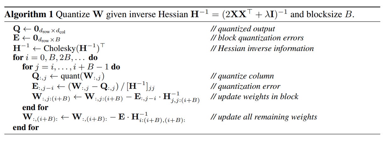
In essence, GPTQ treats quantization as an optimization problem: for each weight it quantizes, it cleverly adjusts the other weights to "soak up" the error, guided by the second-order information from the Hessian matrix.
3. AWQ: Activation-Aware Weight Quantization
AWQ starts from a different insight: not all weights are equally important.
Instead of just looking at the weights themselves, AWQ also looks at the activations that flow through them. It argues that the most important weights are those that are consistently multiplied by large activation values. It finds this small fraction of "salient" weights (often <1% of the total) and leaves them in high precision (FP16), while quantizing the rest aggressively.

A Deep Dive into GPTQ and AWQ Quantization | by Doil Kim
Let's return to the Doil Kim article for a concise summary of AWQ and its contrast with GPTQ.
Please read the sections 'AWQ: Activation-Aware Weight Quantization' and 'GPTQ: Optimal Brain Quantization'. This will solidify your understanding of their distinct philosophies.
GPTQ vs. AWQ: A Summary
| Method | Core Philosophy | Analogy |
|---|---|---|
| GPTQ | Minimize the layer's output reconstruction error. | A careful accountant who, after rounding a number, adjusts other numbers on the balance sheet to keep the total the same. |
| AWQ | Protect the most important weights. | A museum curator who puts the most valuable artifacts behind thicker glass, while giving standard protection to the rest. |
Test your understanding!
You need to deploy a large 70B parameter model, which is ~140GB in its native FP16 format, onto a cluster of A100 GPUs, each with 80GB of VRAM.
- What optimization technique is absolutely essential to make this deployment feasible on single GPUs?
- You are considering both GPTQ and AWQ for 4-bit quantization. In one sentence for each, what is the fundamental principle you would be relying on to preserve the model's accuracy?
Show answer
- 4-bit quantization is essential. It would reduce the model size by approximately 4x, from ~140GB to ~35GB, allowing it to fit comfortably within the 80GB VRAM of a single A100 GPU.
- With GPTQ, you would be relying on its ability to iteratively quantize weights while updating the remaining weights to compensate for the introduced error, thus preserving the layer's overall output. With AWQ, you would be relying on its ability to identify and protect the small subset of critically important weights in higher precision, assuming that preserving these salient weights is sufficient to maintain overall model performance.
Implementation Walkthrough: Quantizing with AutoGPTQ
Now, let's move from theory to practice. We'll walk through the process of quantizing a model using the auto-gptq library. While you won't run the code right now due to setup time, follow the steps closely to understand the workflow. We will quantize the gpt2 model as a simple example.
The following code is adapted from the excellent tutorial in "Making LLMs Lighter".
Step 1: Installation and Setup
First, you would install the necessary libraries. auto-gptq often requires specific CUDA toolkit versions and can be tricky to install, sometimes requiring installation from source.
# Example installation
pip install auto-gptq optimum
Step 2: Load Model, Tokenizer, and Quantization Config
In your Python script, you define the model you want to quantize and configure the quantization parameters.
from transformers import AutoTokenizer, TextGenerationPipeline
from auto_gptq import AutoGPTQForCausalLM, BaseQuantizeConfig

model_id = "gpt2"

# Load the tokenizer
tokenizer = AutoTokenizer.from_pretrained(model_id)

# Define the quantization configuration
quantize_config = BaseQuantizeConfig(
    bits=4,  # Quantize to 4 bits
    group_size=128,  # Group weights in blocks of 128
    damp_percent=0.01, # A parameter for stabilizing Hessian matrix computation
    desc_act=False, # Legacy parameter
)

# Load the unquantized model, passing the config
model = AutoGPTQForCausalLM.from_pretrained(model_id, quantize_config)
bits=4: This is the target bit-width.group_size=128: This is a key parameter. Instead of having one scaling factor for a whole weight matrix, GPTQ groups weights (e.g., 128 at a time) and calculates scaling factors for each group. This significantly improves accuracy over per-tensor quantization.
Step 3: Prepare a Calibration Dataset
GPTQ needs to see some real data to compute the Hessian matrix (H) which guides the quantization process. This is called the calibration dataset. You don't need a huge amount of data; a few hundred samples are often sufficient.
from datasets import load_dataset

# Load a sample of a dataset
data = load_dataset("allenai/c4", "en", split="train[:512]")

# Tokenize the data
tokenized_data = [tokenizer(example['text'], return_tensors='pt') for example in data]
Step 4: Run Quantization
This is the main step. The .quantize() method iterates through the calibration data, computes the Hessians, and applies the GPTQ algorithm layer by layer.
# Run the quantization process
model.quantize(
    tokenized_data,
    batch_size=1,
)
This process can take some time, from minutes for a small model like GPT2 to hours for a 70B model.
Step 5: Save the Quantized Model
Finally, you save the newly quantized model weights and the configuration file. The output is a much smaller model ready for fast inference.
quantized_model_dir = "gpt2-gptq"
model.save_quantized(quantized_model_dir, use_safetensors=True)
tokenizer.save_pretrained(quantized_model_dir)

print(f"Quantized model saved to {quantized_model_dir}")
You now have a directory containing a lightweight, 4-bit version of GPT2 that can be loaded by any inference framework that supports the auto-gptq format.
Conclusion
You've now explored one of the most impactful optimization techniques in the LLM toolkit. Quantization is not just a "nice-to-have"; it's a foundational technology that enables the practical deployment of today's massive language models.
Key Takeaways:
- Quantization's Goal: Reduce model size and inference latency by lowering the numerical precision of weights, at the cost of some potential accuracy degradation.
- The Big Trade-off: The primary challenge is minimizing accuracy loss while maximizing compression and speed gains. This is most effective in memory-bound scenarios.
- PTQ is King: Post-Training Quantization (PTQ) is the standard for LLMs, avoiding the need for costly retraining.
- Leading Methods:
- GPTQ intelligently compensates for quantization error by updating remaining weights, guided by the Hessian matrix.
- AWQ protects a small fraction of "salient" weights (identified via activations) in higher precision.
- Practical Implementation: Libraries like
auto-gptqandbitsandbytesprovide a clear workflow: load a model, define a config, run quantization on a calibration dataset, and save the result.
What's Next?
We have now covered how to choose a serving engine and how to optimize the model itself for inference. The next logical step is to build the application layer around this optimized model. In the upcoming lesson, you will design a robust LLM-powered API endpoint with proper error handling, input validation, and request/response schemas. We'll move from the engine room to the bridge, focusing on the best practices for creating a reliable and user-friendly service.