Cohort Analysis for User Retention

What is Cohort Analysis and Why Does it Matter?

A cohort is a group of users who share a common characteristic. In retention analysis, this characteristic is typically their acquisition date—the month they first signed up or made their first purchase.

Cohort analysis tracks these groups over time to see how many of them remain active. It helps answer critical business questions like:

• Are our newer customers sticking around longer than our older ones?
• Did a specific product change in March improve long-term user engagement?
• How long does it take for a typical customer to stop using our service (churn)?

The final output is usually a table or a heatmap that looks like this:

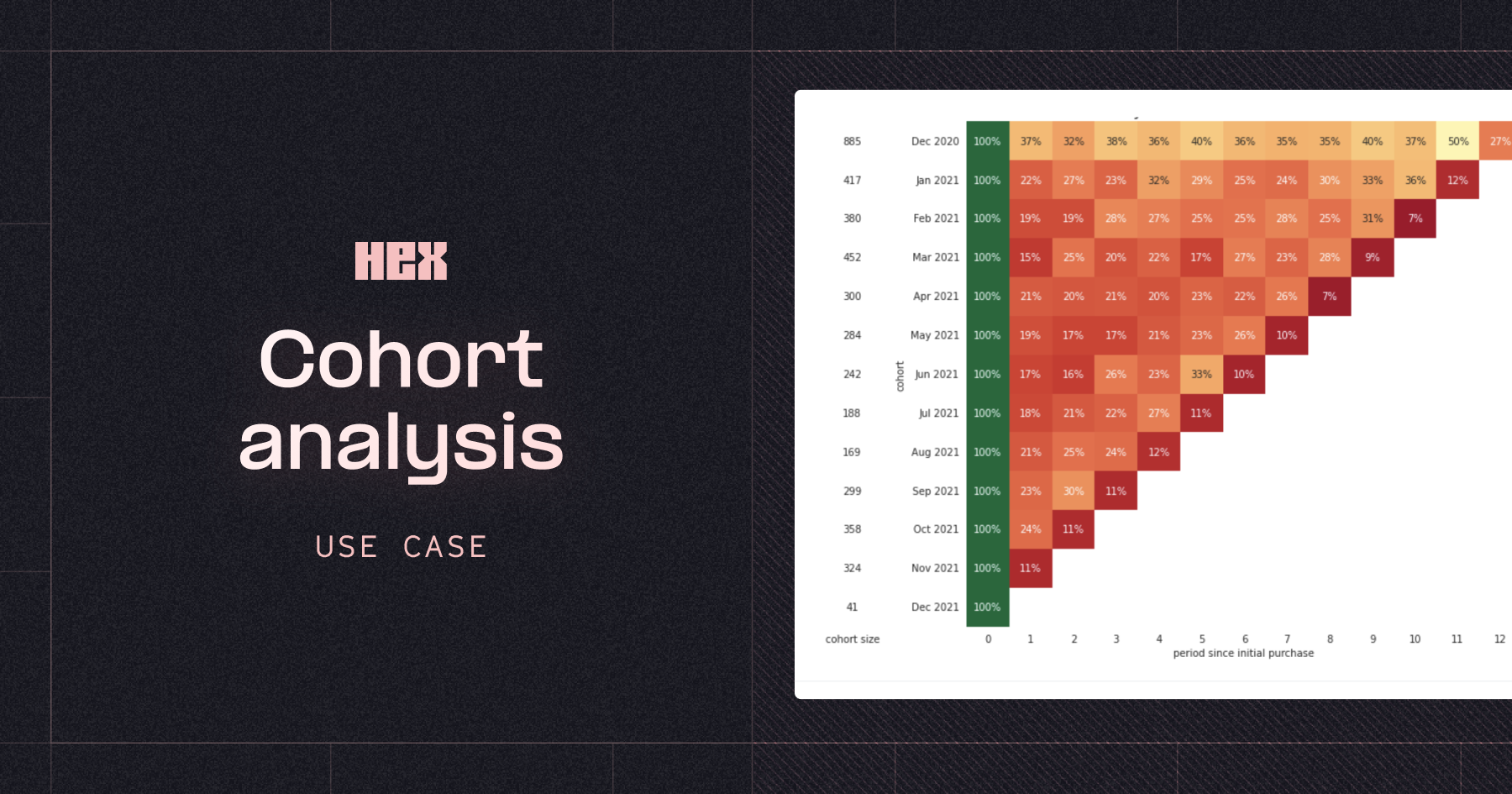
Reading this chart, you can see that for the "Dec 2020" cohort, 100% of users were active in their first month (Month 0), 37% returned in the next month (Month 1), 32% in the month after that (Month 2), and so on.

The Logic: A 3-Step Process

Building a cohort analysis in SQL might seem complex, but it boils down to three logical steps. We'll use Common Table Expressions (CTEs) to organize our query, which you've seen helps make complex logic readable and maintainable.

1. Assign a Cohort to Each Customer: First, we need to find the very first month each customer made a purchase. This "birth month" defines their cohort. We can do this by grouping our transactions by CustomerID and finding the MIN(OrderDate). This step uses the DATE_TRUNC function from our last lesson to ensure we are grouping by month.
2. Calculate the "Age" of Each Transaction: Next, for every transaction a customer makes, we need to calculate how many months have passed since their first purchase. We'll call this the cohort_index or month_number. A transaction in the same month as the first purchase is in month 0, a transaction the next month is in month 1, and so on.
3. Aggregate and Pivot: Finally, we count the number of unique customers for each cohort_month and cohort_index. This gives us the raw data for our retention table. The last (and optional) step is to "pivot" this data to create the matrix format shown in the heatmap above.

This article provides a concise textual summary of this 3-step logic.

Implementing Cohort Analysis in SQL: A Video Walkthrough

Now, let's watch a detailed video that implements this logic step-by-step. The presenter first builds intuition in Google Sheets before translating the entire process into a BigQuery SQL query. The SQL syntax is very similar to what you've used before (PostgreSQL, SQL Server).

This video is the core resource for this lesson. It will walk you through the entire process, from raw data to a final, pivoted retention table.

Synthesizing the Logic into a Single Query

Based on the resources, here is a complete SQL query (in a PostgreSQL/BigQuery dialect) that structures a cohort analysis. It uses CTEs to follow our 3-step process.

WITH 
-- Step 1: Find the first purchase month for each customer to define their cohort
CustomerCohorts AS (
    SELECT
        CustomerID,
        MIN(DATE_TRUNC('month', OrderDate)) AS CohortMonth
    FROM
        Orders
    WHERE 
        CustomerID IS NOT NULL
    GROUP BY
        CustomerID
),

-- Step 2: For each order, calculate the number of months since the customer's first purchase
ActivityByMonth AS (
    SELECT
        o.CustomerID,
        -- Calculate the difference in months between the order date and the cohort month
        DATE_DIFF(
            DATE_TRUNC('month', o.OrderDate), 
            c.CohortMonth, 
            MONTH
        ) AS MonthNumber
    FROM
        Orders o
    JOIN
        CustomerCohorts c ON o.CustomerID = c.CustomerID
),

-- Step 3: Count the number of unique customers for each cohort and month number
CohortRetention AS (
    SELECT
        c.CohortMonth,
        a.MonthNumber,
        COUNT(DISTINCT a.CustomerID) AS ActiveCustomers
    FROM
        ActivityByMonth a
    JOIN
        CustomerCohorts c ON a.CustomerID = c.CustomerID
    GROUP BY
        1, 2
)

-- Final Selection: Calculate retention percentages
SELECT
    r.CohortMonth,
    -- Get the initial cohort size (customers from MonthNumber = 0)
    FIRST_VALUE(r.ActiveCustomers) OVER (PARTITION BY r.CohortMonth ORDER BY r.MonthNumber) AS CohortSize,
    r.MonthNumber,
    r.ActiveCustomers,
    -- Calculate retention percentage
    (r.ActiveCustomers::decimal / FIRST_VALUE(r.ActiveCustomers) OVER (PARTITION BY r.CohortMonth ORDER BY r.MonthNumber)) * 100 AS RetentionPercentage
FROM
    CohortRetention r
ORDER BY
    1, 3;

This query produces a "long" table format. To get the "wide" pivoted format, you would use your database's PIVOT function or conditional aggregation with CASE statements on this final result. The video you watched demonstrates the PIVOT approach.

A Practical Note: Data Cleaning

The video and queries assume the data is relatively clean. In a real-world scenario, you would first need to handle issues like NULL customer IDs, returned orders (which might have negative quantities), and duplicate transaction records.

The following video provides an excellent example of this preliminary cleaning phase before cohort analysis even begins.

This cleaning step is vital for accuracy. For instance, if you don't remove NULL customer IDs, you might group all those sales into a single, meaningless "NULL cohort".

Conclusion

Congratulations! You've just learned how to build one of the most valuable reports in business analytics. By structuring a cohort analysis, you can provide deep insights into customer behavior, product stickiness, and the overall health of a business.

Key Takeaways:

• Cohort analysis groups users by their acquisition date and tracks their activity over subsequent periods to measure retention.
• The process can be broken down into three logical steps in SQL using CTEs:
  1. Define Cohorts: Find each customer's first activity date (MIN + GROUP BY).
  2. Calculate Activity Age: For each activity, find the time difference from the customer's cohort date (DATE_DIFF).
  3. Aggregate: Count unique customers per cohort and age (COUNT(DISTINCT) + GROUP BY).
• The final result can be a "long" table of percentages or pivoted into a "wide" matrix for visualization as a heatmap.
• Real-world analysis always begins with thorough data cleaning to ensure your results are accurate.

Next Lesson Preview:

In the video on data cleaning, you saw the importance of handling missing values. In our next lesson, we will focus specifically on that. You will learn how to handle NULL values in analytical queries using functions like COALESCE and NULLIF to ensure accurate aggregations. This will equip you with the tools to make your analyses more robust and reliable.