Hello! In our previous lesson, we focused on creating dropdown lists to standardize data entry, a crucial step in maintaining data integrity for accounting tasks. By ensuring inputs are consistent, you've laid the groundwork for reliable analysis.
Today, we'll take the next logical step and learn how to make that data speak to you visually. We will explore conditional formatting, an Excel feature that automatically changes the appearance of cells based on the data they contain. Your goal for this lesson is to master Excel's built-in conditional formatting tools to highlight key financial figures, spot trends, and flag important information at a glance. Instead of just looking at a wall of numbers, you'll learn to make your spreadsheets automatically draw attention to what matters most.
From Data to Insight: The Power of Visual Analysis
In accounting and finance, quick and accurate analysis is paramount. Conditional formatting transforms a static report into a dynamic dashboard. It's not about making things look pretty; it's about building an automated system that helps you identify risks, opportunities, and errors instantly.
Imagine an inventory list where items with low stock are automatically highlighted in yellow, or a sales report where the highest-performing products have a green data bar next to them. This is the power of conditional formatting.
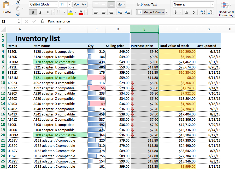
As someone with a background in commerce, you understand concepts like liquidity and the fundamental accounting equation. Conditional formatting can bring these concepts to life directly within your models.
How to Use Conditional Formatting for Cash Flow Models
This article from the Corporate Finance Institute (CFI) perfectly illustrates the strategic value of conditional formatting in a professional financial context.
Please read the introductory section, "The Value of Conditional Formatting in Cash Flow Models." It explains why this tool is essential for spotting risks like cash shortfalls in complex financial models.
Applying Built-in Formatting Rules
Excel's conditional formatting tools are found on the Home tab of the ribbon. Most of your needs can be met with the powerful built-in options, which we'll explore now. We'll look at the main categories: Highlight Cells Rules, Top/Bottom Rules, Data Bars, Color Scales, and Icon Sets.
This video provides a great overview of these features, which we will break down in more detail.
Excel Conditional Formatting in Depth
This in-depth tutorial from the "Technology for Teachers and Students" channel provides clear examples of the different types of conditional formatting.
Watch the introduction from this timestamp to get a clear definition of what conditional formatting is and where to find it.
1. Highlight Cells Rules
This is the most common and direct type of conditional formatting. It allows you to format cells that meet specific criteria, such as being greater than a certain number, containing specific text, or being equal to a value.
For an accountant, this is invaluable for:
- Flagging budget overruns: Highlight all expense cells
Greater Thanthe budgeted amount. - Identifying duplicate entries: Highlight
Duplicate Valuesin a list of invoice numbers to find potential errors. - Categorizing transactions: Highlight cells with
Text that Contains"Interest" to quickly see all interest-related payments.
A classic accounting application is the balance sheet check. You can create a cell that shows "Okay" if Assets = Liabilities + Equity and "Error" otherwise. Conditional formatting can then make this check impossible to ignore.
How to Use Conditional Formatting for Cash Flow Models
Let's return to the CFI article to see a practical demonstration of the "Equal To" rule.
Read the section "Highlighting the Balance Sheet Check." This shows you how to apply two rules: one to make "Okay" green and another to make "Error" red. This is a fundamental technique in financial modeling.
2. Top/Bottom Rules
While "Highlight Cells Rules" looks for absolute values, "Top/Bottom Rules" are relative. They format cells based on their rank within a selected range. You can instantly find:
- The Top 10 best-selling products.
- The Bottom 10% of stores by performance.
- All sales figures that are Above Average for the quarter.
This is extremely useful for performance analysis and identifying outliers without needing to sort or filter the data first.
Applying Conditional Formatting in Microsoft Excel
This clip from Simon Sez IT gives a quick and clear demonstration of applying a Top/Bottom rule.
Watch the short segment on highlighting top items to see how quickly you can identify the highest values in a dataset.
3. Data Bars
Data bars add a small bar chart inside each cell, with the length of the bar corresponding to the cell's value relative to others in the range. This provides a powerful and immediate visual comparison of magnitude. This is perfect for presenting columns like 'Sales', 'Inventory Quantity', or 'Turnover' where you want to see at a glance which items are the largest.
Master Excel Conditional Formatting: Build Dynamic Data Reports ...
This article from "The Excel Bee" clearly explains how data bars can make large numbers easier to interpret.
Read the section "In-Cell Data Bars," which shows how to apply them to a "Turnover" column in a stock data report.
4. Color Scales
Color scales, or "heat maps," apply a color gradient to a range of cells. This is ideal for visualizing data that has a spectrum from "good" to "bad" or "low" to "high." For example, a common green-yellow-red scale instantly communicates performance, just like a traffic light:
- Green: High values (e.g., high profit margins, high sales growth).
- Yellow: Average values.
- Red: Low values (e.g., low profit margins, negative growth).
This is highly effective for analyzing financial ratios or key performance indicators (KPIs) across different periods or business units.
Applying Conditional Formatting in Microsoft Excel
Let's return to the Simon Sez IT video to see how color scales work.
Watch the segment from this timestamp. Notice how different color schemes can be used to tell different stories with the data.
5. Icon Sets
Icon sets place a small icon in each cell to categorize its value. Common sets include:
- Directional arrows: Up, down, or sideways arrows are perfect for showing trends or variances (e.g., sales up from last month).
- Traffic lights or flags: These are great for indicating status (e.g., green for 'On Track', yellow for 'Needs Review', red for 'Overdue').
- Ratings: Star or bar ratings can represent performance levels.
A key skill is customizing these icon sets. For instance, you might only want to show an arrow if a variance is significant (e.g., greater than 5%), keeping the report clean.
Master Excel Conditional Formatting: Build Dynamic Data Reports ...
This final reading from "The Excel Bee" demonstrates a powerful customization technique for icon sets.
Read the section "Custom Icon Sets for Daily Movers." Pay close attention to how the rule is edited to only show icons for significant movements, which makes the report much more focused and professional.
Conclusion
In this lesson, you've learned to transform your raw financial data into a dynamic visual report using Excel's built-in conditional formatting tools. By automatically highlighting key figures, you can analyze information faster and more intuitively, a critical skill for any accounting professional.
Key Takeaways:
- Conditional formatting is an essential tool for visual data analysis, helping to spot trends, outliers, and risks.
- Highlight Cells Rules are used for formatting cells based on their specific content (e.g., value is greater than X, text contains "Expense").
- Top/Bottom Rules are used to identify relative performers within a dataset (e.g., top 10 products).
- Data Bars, Color Scales, and Icon Sets provide powerful in-cell visualizations to compare magnitude and indicate status at a glance.
- Customizing these rules, such as changing thresholds for icon sets, is key to creating clean and effective reports.
In our next lesson, we will unlock even more power by moving beyond the built-in presets. You will learn how to create a conditional formatting rule for an entire table row based on a custom formula. This will allow you to do things like highlight an entire invoice record in red if its status, chosen from a dropdown list, is "Overdue."