Consolidate Data with 3-D References

The Problem: Consolidating Data Manually

Imagine you have a workbook with separate sheets for your company's sales in January, February, March, and April. Each sheet has the exact same layout, listing products and their sales figures. On a "Summary" sheet, you want to calculate the total sales for each product over the four months.

The tedious, manual approach would be to write a formula like this for the first product:
=Jan!B2 + Feb!B2 + Mar!B2 + Apr!B2

While this works, it has major drawbacks:

• Inefficient: It's time-consuming to click on each sheet, especially if you have twelve months or more.
• Error-Prone: It's easy to miss a sheet or click the wrong cell.
• Static: If you add a "May" worksheet, you must manually go back and edit every single summary formula.

This manual method is the opposite of the automation we are aiming for. There is a far more elegant solution.

The Solution: 3-D References

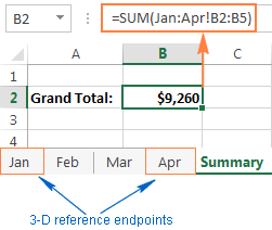
A 3-D reference allows you to refer to the same cell or range of cells across a range of worksheets. Instead of adding each sheet individually, you specify the start and end sheets, and Excel includes everything in between.

The syntax looks like this: =FUNCTION(StartSheet:EndSheet!CellRange)

For our example, the formula becomes: =SUM(Jan:Apr!B2:B5)

This single formula adds up the values in the range B2:B5 across all worksheets from "Jan" through "Apr".

For a formal definition, the official Microsoft documentation provides a concise overview.

How to Create a 3-D Reference

Now, let's walk through creating one. While you can type them manually, it's often easier and more accurate to create them by clicking. The process involves starting your formula, selecting the first sheet, holding the SHIFT key, and then selecting the last sheet in your range.

This video by Leila Gharani provides an excellent demonstration, contrasting the inefficient manual method with the streamlined 3-D formula approach.

The key prerequisite, as mentioned in the video, is that all worksheets you include in the reference must have the same structure. The data you want to aggregate must be in the same cell or range on every sheet.

The Real Power: Dynamic Updates

The most significant advantage of 3-D references is that they are dynamic. If you insert a new worksheet anywhere between the start and end sheets of your reference, Excel automatically includes its data in the calculation.

Imagine you have the summary formula =SUM(Jan:Apr!B2). If you add a new "May" sheet and place it between "Apr" and "Jan", the formula won't see it. But if you drag the "May" sheet to be between "Jan" and "Apr", the formula result updates instantly to include May's data. No manual editing is required.

This makes it incredibly easy to maintain rolling reports. You can set up your summary once, and as you add new monthly or quarterly sheets, your summary report stays up-to-date.

Important Considerations and Pitfalls

While powerful, 3-D references require careful handling to ensure data integrity.

1. Moving and Deleting Sheets

The formula is dependent on the physical order of the sheets.

• Moving a sheet out: If you move a worksheet that was between the endpoints to a location outside of them, its values are removed from the calculation.
• Deleting a sheet: If you delete a worksheet from within the range, its values are removed.
• Deleting an endpoint: If you delete the start or end sheet (e.g., you delete the "Jan" sheet from Jan:Apr!B2), the range automatically shrinks (e.g., to Feb:Apr!B2).

2. Accidental Inclusion

A common pitfall is accidentally dragging an unrelated worksheet into the middle of your 3-D reference range. Because the formula includes everything between the endpoints, this can silently add incorrect data to your totals and corrupt your summary report.

The video from Leila Gharani demonstrates this pitfall perfectly.

3. Function Compatibility

Not all Excel functions support 3-D references. They are primarily for simple aggregation functions. This article from Chris Menard clearly demonstrates the recommended way to use the SUM function.

The most common compatible functions you will use are:

• SUM
• AVERAGE
• COUNTA (counts non-empty cells)
• COUNT (counts cells with numbers)
• MAX
• MIN

Making Formulas More Readable with Named Ranges

For complex workbooks, you can make your 3-D formulas much easier to read and manage by assigning a name to the 3-D reference itself. For example, you could define the name Q1_Sales to refer to Jan:Mar!B2:B10. Then, your formula simply becomes =SUM(Q1_Sales). This is excellent practice for building clean and maintainable financial models.

Conclusion

You have now learned how to use 3-D references to efficiently consolidate data from multiple, identically structured worksheets. This is a fundamental skill for automating summary reports in accounting, saving you from tedious and error-prone manual calculations.

Key Takeaways:

• Purpose: Use 3-D references to aggregate data (e.g., SUM, AVERAGE) from the same cell or range across multiple worksheets.
• Syntax: The format is FUNCTION(StartSheet:EndSheet!CellRange).
• Dynamic Nature: New sheets inserted between the start and end sheets are automatically included in calculations.
• Prerequisite: All referenced worksheets must have an identical layout for the formula to work correctly.
• Pitfall: Be cautious not to place unrelated worksheets within your referenced range, as they will be included in the calculation.

In this module, we've covered data validation, conditional formatting, charting, and now, 3-D references. These tools are all about ensuring data integrity and presenting it clearly.

In our next module, we will explore an even more powerful and flexible tool for summarizing data: PivotTables. While 3-D references are perfect for identically structured sheets, PivotTables allow you to summarize and analyze large, raw datasets that are all in a single list, opening up a new world of dynamic reporting.