Welcome to the final lesson of our module on summarizing data. So far, you've learned to build powerful summary reports using PivotTables, group data by time periods, create interactive filters with Slicers, and even add your own custom formulas with calculated fields. We've built the analytical engine; now it's time to create the visual dashboard.
This lesson focuses on PivotCharts. A PivotChart is a dynamic chart that is directly linked to a PivotTable. This connection is what makes it so powerful for accounting and financial analysis. Instead of creating a static chart that you have to manually update, a PivotChart automatically reflects any changes you make to your PivotTable—whether it's filtering by region, drilling down into a different quarter, or updating the underlying data.
By the end of this lesson, you will be able to create and format a PivotChart to visually analyze financial trends and comparisons, transforming your numerical summaries into compelling visual stories.
From Table to Trendline: The Power of PivotCharts
A picture is worth a thousand numbers, especially in a management meeting. While a PivotTable is excellent for detailed analysis, a PivotChart provides an immediate, high-level understanding of trends, comparisons, and outliers. Because your background is in commerce, you know that analyzing trends in revenue, expenses, or profit is a cornerstone of financial management. A PivotChart is the Excel tool designed for exactly that.
The key thing to remember is that the PivotTable and PivotChart are a team. The PivotTable does the data crunching, and the PivotChart visualizes the results. You cannot have a PivotChart without a PivotTable.
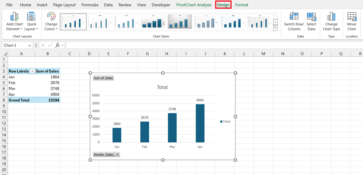
Creating Your First PivotChart
Let's begin by creating a basic PivotChart. The process is straightforward and builds directly on the skills you've already acquired. You start with a PivotTable and simply add a visual layer on top of it.
The following guide uses a dataset of government expenditures to demonstrate how to build a PivotTable and then create a line chart from it. This is a great, visual step-by-step walkthrough of the fundamental process.
[PDF] Transaction Analysis Using Excel Pivot Tables and Charts
This PDF tutorial provides a clear, slide-by-slide guide to creating a PivotTable and its corresponding PivotChart.
Please start reading from slide 66, titled "Req 6". Follow the steps from slide 66 to slide 74. Pay close attention to these key steps: Slide 67: Notice that you can insert both a PivotChart and PivotTable at the same time from the Insert tab. Slide 69: You build the chart by arranging fields in the PivotTable Fields pane, just as you would for a regular PivotTable. Slide 71-72: You can easily change the chart type after it has been created.
Visualizing Trends Over Time
One of the most common tasks for an accountant is analyzing performance over a period. A line chart is perfect for this, as it clearly shows trends, seasonality, and growth. Let's create a PivotChart that tracks monthly revenue.
This process combines several skills you've learned: creating a PivotTable, grouping dates by month and year, and now, inserting a PivotChart.
The following video provides a concise demonstration of this entire workflow, from raw data to a finished trendline chart.
Compare Years in Excel Pivot Chart - Step by Step Line Chart
This video from Contextures Inc. walks through creating a time-series PivotChart.
Watch these three segments to see the process unfold: First, see how the PivotTable is created from a structured table from the initial setup. Next, watch how a line PivotChart is inserted from the PivotTable from inserting the chart. Finally, observe the crucial step of grouping the date field to make the chart readable, from grouping the dates.
Building an Interactive Dashboard with Slicers
The true power of a PivotChart is unlocked when you combine it with Slicers. This transforms a static report into an interactive dashboard, allowing you or your manager to explore the data by clicking buttons.
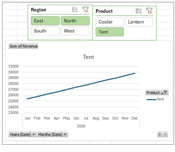
Let's build on the time-series chart by adding Slicers for 'Region' and 'Product'. This will allow a user to instantly see revenue trends for any combination of product and region. The Journal of Accountancy provides a perfect guide for this.
Create interactive dashboards with Excel PivotCharts and ...
This article from the Journal of Accountancy details how to build a professional, interactive dashboard.
Please read the following sections: Start with "Create the PivotTable". This recaps the process of creating the table and inserting the chart. Continue to "Add interactive filters". This explains how to insert and format Slicers that control the chart. Finally, look at the result in the section that begins with "The functional dashboard".
After following those steps, you will have a functional dashboard like the one below, where clicking on "East" or "Tent" immediately filters the line chart.
Polishing Your PivotChart for Presentation
Like any chart, a PivotChart needs some formatting to be ready for a report or presentation. There are two common adjustments you'll want to make.
- Hiding Field Buttons: The gray buttons on the chart (e.g., "Months (Date)") are useful for quick filtering but can clutter the final visual. You can hide them for a cleaner look.
- Renaming Legend Entries: The chart legend might automatically display "Sum of Revenue" when all you want is "Revenue". You can fix this by renaming the field in the PivotTable.
The following video shows exactly how to perform these two essential formatting tasks.
Pivot Tables: MUST-KNOW for Business & Finance Professionals
This video from Kenji Explains covers essential formatting tips for PivotCharts.
Watch the segment from this demonstration. It shows you how to hide the field buttons and how to edit the value field settings to clean up the legend text. Notice the useful trick of adding a space to the name if Excel says the name already exists.
Advanced Analysis: Year-Over-Year Comparison
A powerful analytical view is to compare different years against each other on the same monthly axis (e.g., January's sales for 2025 vs. 2026). You can achieve this with a simple drag-and-drop in your PivotTable field list.
By moving the 'Years' field from the Rows area to the Columns (or Legend) area, you instruct the PivotChart to draw a separate line for each year. This makes year-over-year comparisons incredibly clear.
This final video clip demonstrates this specific, powerful technique.
Compare Years in Excel Pivot Chart - Step by Step Line Chart
This clip shows how to create a year-over-year comparison chart.
Watch the short segment from this video. Pay attention to how dragging the 'Years' field into the 'Columns' area instantly changes the chart from a single continuous timeline into a multi-line comparative chart.
Conclusion
You have now completed the journey from raw data to a fully interactive visual dashboard. This is a critical skill for any modern accountant, enabling you to present financial data in a way that is clear, insightful, and easy to explore.
Key Takeaways:
- PivotCharts are dynamic visualizations directly linked to a PivotTable.
- They are created by selecting a PivotTable and using the PivotChart button on the PivotTable Analyze tab.
- The chart's appearance is controlled by the PivotTable's field layout; changing the table instantly changes the chart.
- Combining PivotCharts with Slicers creates powerful interactive dashboards.
- For professional presentation, you can hide field buttons and customize legend names.
- To create a year-over-year comparison, place your time unit (e.g., Months) in the Rows/Axis area and the 'Years' field in the Columns/Legend area.
This lesson concludes our module on summarizing data with PivotTables. You have mastered one of the most powerful analytical tools in Excel.
In our next module, we will shift gears to a more structured form of reporting: Building Dynamic Financial Statements. We will take the core principles of data handling you've learned and apply them using functions like SUMIFS to construct a formal Income Statement and Balance Sheet from a trial balance, a foundational task in accounting.