Entropy and Gini Impurity: Measuring Node Impurity for Tree Splits

Hello! In our last two lessons, we established what a decision tree is and explored the critical trade-off between underfitting and overfitting. We learned that to prevent a tree from becoming too complex and memorizing the training data, we need to control its growth. This naturally leads to a crucial question: if the tree has to make a choice at each step, how does it decide which feature makes for the "best" split?

Today's lesson will answer that question directly. Your learning outcome is to explain the formulas for Entropy and Gini Impurity, and demonstrate their use in measuring node impurity for tree splits. These two metrics are the mathematical engine a decision tree uses to build itself, quantifying the "goodness" of a potential split. Understanding them is key to a deeper grasp of tree-based models and is a frequent topic in exam questions.

1. The Goal of a Split: Maximizing Purity

Imagine a group of data points at a node in our tree, each labeled either "Survived" or "Died."

If all data points have the same label (e.g., all "Survived"), we can say the node is pure. No further splitting is needed.
If the node contains a mix of labels (e.g., 50% "Survived," 50% "Died"), it is impure or disordered.

The fundamental goal of the decision tree algorithm at each step is to find a split (a question about a feature, like "Is Age > 42?") that results in child nodes that are, on average, purer than the parent node was. To do this, the algorithm needs a way to numerically measure this impurity. Let's explore the two most common methods.

2. Method 1: Entropy and Information Gain

The concept of entropy originally comes from physics and information theory, where it's a measure of disorder or uncertainty. In the context of decision trees, it measures the impurity of a node. A great way to build intuition for entropy is to think about it as "average surprise."

This video from the StatQuest channel explains this idea beautifully.

Entropy (for data science) Clearly Explained!!!

This video, "Entropy (for data science) Clearly Explained!!!", breaks down the concept of entropy starting from the intuitive idea of "surprise."

Please watch the following segments: The relationship between probability and surprise. How surprise is calculated using logarithms. The definition of entropy as "average" or "expected" surprise. The standard formula for entropy. Finally, see it applied in the chicken example, which shows how entropy quantifies the disorder in a group.

As the video explains, the standard formula for entropy in a node with $c$ different classes is:
$H (S) = - \sum_{i = 1}^{c} p_{i} lo g_{2} (p_{i})$
Where $p_{i}$ is the proportion (or probability) of samples belonging to class $i$ in that node.

Key properties of Entropy for a two-class problem:

Entropy = 0 when a node is perfectly pure (e.g., all samples are "Survived," so $p_{S} = 1, p_{D} = 0$ ). There is no surprise.
Entropy = 1 when a node is maximally impure (e.g., a 50/50 split of "Survived" and "Died"). This is the state of maximum uncertainty.

The decision tree doesn't just calculate the entropy of the child nodes; it calculates the Information Gain (IG), which is the reduction in entropy achieved by making a split.

$Information Gain = Entropy (parent) - Weighted Average Entropy (children)$

The algorithm calculates the Information Gain for every possible split and chooses the one that maximizes it. A high Information Gain means the split was very effective at creating purer, more organized child nodes.

3. Method 2: Gini Impurity

Gini Impurity is an alternative metric that serves the same purpose as entropy but is computationally faster because it doesn't involve logarithmic calculations.

The intuition behind Gini Impurity is the probability of incorrectly classifying a randomly chosen data point from a node, if you were to label it randomly according to the class distribution within that node.

The StatQuest channel also provides an exceptionally clear walkthrough of calculating Gini Impurity.

Decision and Classification Trees, Clearly Explained!!!

This clip is from the video "Decision and Classification Trees, Clearly Explained!!!". It introduces the need to quantify impurity and then details the Gini Impurity calculation.

Watch the following two segments: The introduction to impure leaves and the need for a metric like Gini Impurity. A step-by-step guide to calculating the Gini Impurity for a split.

The formula for Gini Impurity is:
$G ini (S) = 1 - \sum_{i = 1}^{c} p_{i}^{2}$
Where, again, $p_{i}$ is the proportion of samples of class $i$ .

Key properties of Gini Impurity for a two-class problem:

Gini Impurity = 0 when a node is perfectly pure.
Gini Impurity = 0.5 when a node is maximally impure (a 50/50 split).

Similar to Information Gain, the algorithm calculates the weighted average Gini Impurity of the child nodes resulting from a split. The algorithm then chooses the split that results in the lowest weighted Gini Impurity. This is equivalent to maximizing the "Gini Gain," or the reduction in impurity.

4. Entropy vs. Gini Impurity: A Quick Comparison

For an exam, you might be asked to compare these two methods. In practice, they are very similar and often lead to almost identical trees.

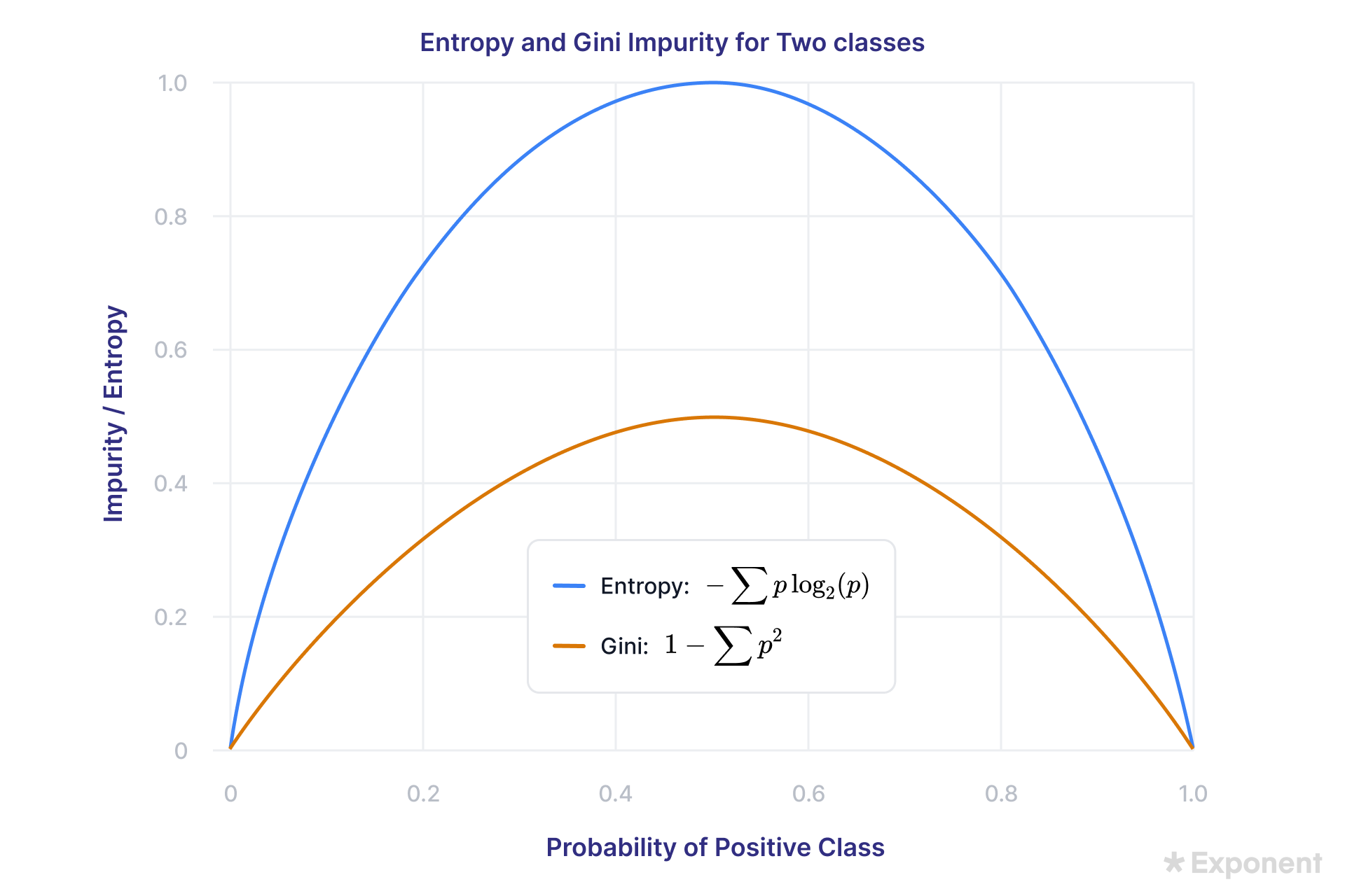
This graph compares the values of Entropy and Gini Impurity for a two-class problem. Both measures are 0 when the probability of the positive class is 0 or 1 (pure node) and reach their maximum when the probability is 0.5 (maximally impure node).

The following reading summarizes the key differences for an interview or exam context.

Mastering ML Interviews: Decision Trees Explained

This article section directly answers the question of how Gini Impurity and Entropy compare.

Please read the answer to question 4, advantages and disadvantages.

In summary:

Gini Impurity is computationally faster as it avoids logarithms. It is the default in many popular libraries like scikit-learn.
Entropy has a stronger foundation in information theory. It can be slightly more sensitive to creating balanced splits.

5. Practical Application: Solving an Exam Problem

Let's apply these concepts to a typical exam-style problem. The goal is to identify which of two possible splits is better by calculating the reduction in impurity.

This image presents a problem with a small dataset of 15 Titanic cases (S for 'Survived', D for 'Died'). We must assess which of two splits, 'Age>42' or 'Ticket>18', leads to a higher reduction in impurity.

Let's use Gini Impurity to solve this.

First, calculate the Gini Impurity of the parent node (the full dataset of 15 cases).

Cases: 6 Survived (S), 9 Died (D).
Proportions: $p_{S} = 6/15 = 0.4$ , $p_{D} = 9/15 = 0.6$ .
$G in i_{p a r e n t} = 1 - (p_{S}^{2} + p_{D}^{2}) = 1 - (0. 4^{2} + 0. 6^{2}) = 1 - (0.16 + 0.36) = 1 - 0.52 = 0.48$ .

Split 1: Age > 42

Left Child (Age <= 42): 10 cases (3S, 7D).
- $p_{S} = 3/10 = 0.3, p_{D} = 7/10 = 0.7$ .
- $G in i_{l e f t} = 1 - (0. 3^{2} + 0. 7^{2}) = 1 - (0.09 + 0.49) = 1 - 0.58 = 0.42$ .
Right Child (Age > 42): 5 cases (3S, 2D).
- $p_{S} = 3/5 = 0.6, p_{D} = 2/5 = 0.4$ .
- $G in i_{r i g h t} = 1 - (0. 6^{2} + 0. 4^{2}) = 1 - (0.36 + 0.16) = 1 - 0.52 = 0.48$ .
Weighted Average Gini:
$(\frac{10}{15} \times 0.42) + (\frac{5}{15} \times 0.48) = (0.67 \times 0.42) + (0.33 \times 0.48) = 0.28 + 0.16 = 0.44$
Gini Gain (Reduction in Impurity): $G in i_{p a r e n t} - G in i_{w e i g h t e d} = 0.48 - 0.44 = 0.04$ .

Split 2: Ticket > 18

Left Child (Ticket <= 18): 8 cases (2S, 6D).
- $p_{S} = 2/8 = 0.25, p_{D} = 6/8 = 0.75$ .
- $G in i_{l e f t} = 1 - (0.2 5^{2} + 0.7 5^{2}) = 1 - (0.0625 + 0.5625) = 1 - 0.625 = 0.375$ .
Right Child (Ticket > 18): 7 cases (4S, 3D).
- $p_{S} = 4/7 \approx 0.57, p_{D} = 3/7 \approx 0.43$ .
- $G in i_{r i g h t} = 1 - (0.5 7^{2} + 0.4 3^{2}) = 1 - (0.325 + 0.185) = 1 - 0.51 = 0.49$ .
Weighted Average Gini:
$(\frac{8}{15} \times 0.375) + (\frac{7}{15} \times 0.49) = (0.53 \times 0.375) + (0.47 \times 0.49) = 0.20 + 0.23 = 0.43$
Gini Gain (Reduction in Impurity): $G in i_{p a r e n t} - G in i_{w e i g h t e d} = 0.48 - 0.43 = 0.05$ .

Conclusion: Split 2 (Ticket > 18) provides a slightly higher reduction in Gini impurity (0.05 vs 0.04). Therefore, the decision tree algorithm would choose Split 2. The same process would be followed using Entropy and Information Gain, and it would likely lead to the same conclusion.

Conclusion

In this lesson, we demystified the process by which a decision tree selects its splits. You now understand the core mechanics driving the tree's construction.

Here are your key takeaways for the exam:

Decision trees create splits by choosing the feature and threshold that result in the purest possible child nodes.
Impurity is a measure of the disorder or mixedness of classes within a node.
Entropy measures impurity based on the concept of "average surprise," with a maximum of 1 for a two-class problem. The goal is to find the split that maximizes Information Gain.
Gini Impurity measures impurity based on the probability of misclassification, with a maximum of 0.5 for a two-class problem. The goal is to find the split that minimizes the weighted average Gini impurity.
While their formulas differ, both methods are conceptually similar and usually produce comparable results, but Gini is computationally faster.

We now have a solid understanding of how a single, powerful decision tree is built. In our next lesson, we will explore Ensemble Learning, a technique that combines many simple decision trees to create models that are far more accurate and robust than any single tree could be on its own.