Composing JAX Transformations

1. A Shift in Perspective: From Tapes to Function Composition

Before diving into specific patterns, it's worth taking a moment to appreciate the conceptual shift that JAX's composability represents. In PyTorch, you define tensors and operations, which implicitly build a dynamic computation graph (a "tape"). Then, you call .backward() on a scalar output, which triggers a traversal of this graph to compute gradients.

JAX operates differently. It transforms entire Python functions into new Python functions. jax.grad(f) doesn't run f; it returns a new function g that computes the gradient of f. Likewise, jax.jit(g) returns a new, compiled function h. The process of "training" in JAX is about composing these transformations to build the exact function you need (e.g., a JIT-compiled, batched, gradient computation function) and then executing it.

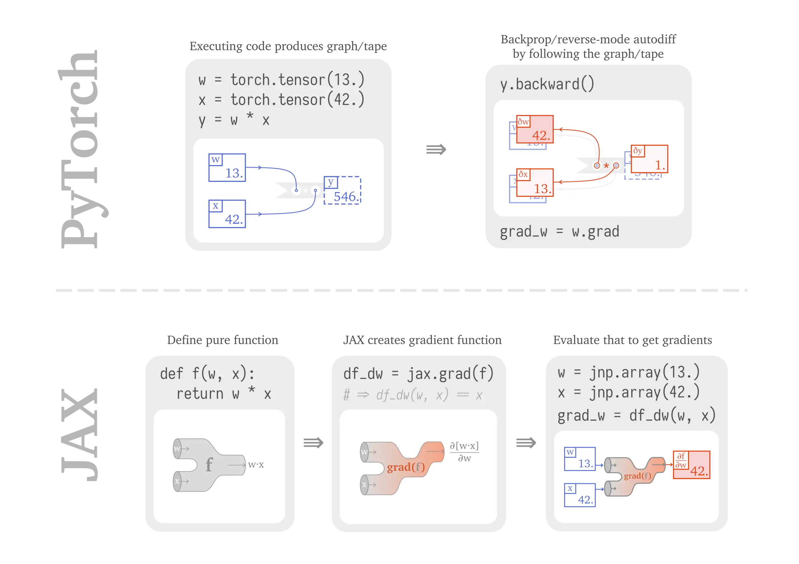
This functional approach is what enables the flexible and predictable composition we'll explore now.

2. The Core Patterns: grad and vmap

The interplay between grad and vmap is central to most machine learning workflows. There are two primary ways to combine them, each serving a distinct and important purpose.

Pattern 1: Gradient of a Batch (grad of a vmap'd computation)

This is the most common pattern in deep learning. You want to compute a single loss value for an entire batch of data (e.g., the mean cross-entropy), and then compute the gradient of that scalar loss with respect to the model parameters.

The logical flow is:

1. Use vmap to apply your model to a batch of inputs, producing a batch of outputs.
2. Compute a scalar loss from the batched outputs and batched targets.
3. Use grad to differentiate this scalar loss.

The result is a single gradient pytree, representing the average gradient over the batch, ready to be passed to an optimizer.

# Conceptual example
# f is a function for a single example, e.g., a model's forward pass
# loss_fn is a per-example loss
def batch_loss(params, inputs, targets):



  # 1. Apply model to a batch of inputs
  predictions = jax.vmap(f, in_axes=(None, 0))(params, inputs)



  # 2. Compute loss for each example, then average
  per_example_loss = jax.vmap(loss_fn)(predictions, targets)
  return jnp.mean(per_example_loss)




# 3. Differentiate the batch loss
grad_fn = jax.grad(batch_loss)



# Calling grad_fn(params, batch_inputs, batch_targets) gives one gradient.

In practice, the vmap is often applied to the model, and the loss function naturally operates on batches, making the code even cleaner.

Pattern 2: Batch of Gradients (vmap of a grad'd computation)

What if you need the gradient for each individual example in the batch? This is known as computing per-example gradients. This is crucial for more advanced techniques like differential privacy (adding noise to per-example gradients), influence functions, and certain meta-learning algorithms.

JAX makes this remarkably expressive: you simply reverse the order of transformations.

1. Use grad to create a function that computes the gradient of the loss for a single example.
2. Use vmap to apply this gradient function across the entire batch of data.

# Conceptual example
def single_example_loss(params, input, target):
  prediction = f(params, input)
  return loss_fn(prediction, target)




# 1. Get gradient function for a single example
single_grad_fn = jax.grad(single_example_loss)




# 2. vmap this gradient function
per_example_grad_fn = jax.vmap(single_grad_fn, in_axes=(None, 0, 0))




# Calling per_example_grad_fn(params, batch_inputs, batch_targets) returns a
# pytree of gradients, where each leaf has an added leading 'batch' dimension.

This ability to "vmap the grad" is a direct consequence of JAX's composable design. Let's see this highlighted in a talk by JAX creator Matt Johnson.

3. The Final Layer: jit for Performance

Once you've composed grad and vmap to define your desired computation, you'll almost always want to wrap the entire thing in jax.jit. This tells the XLA compiler to take the whole computational graph—forward pass, loss calculation, and backward pass—and optimize it into a single, highly efficient kernel.

The rule of thumb is to apply jit as the outermost transformation.

• Good: jit(grad(batch_loss))
• Bad: grad(jit(batch_loss))

Why? jit works by tracing a function to create a static computation graph. You want to give it the largest possible graph to analyze and optimize. Jitting the entire gradient computation allows XLA to perform optimizations like fusion, where it can merge the forward and backward pass operations, eliminating intermediate memory allocations and dramatically improving performance. If you were to jit only the forward pass, the backward pass generated by grad would run in eager mode, negating much of the benefit.

4. A Real-World Training Step

Let's see how these pieces come together in a practical training step. The nanoJAXGPT project is a from-scratch implementation of a GPT-style model in JAX and Equinox, making it a perfect case study for your goals.

5. The Sky's the Limit: Arbitrary Composition

The examples we've seen are the bread and butter of deep learning in JAX. However, the system is designed for much more. Because the interpreters for the transformations are themselves written in a transformable subset of Python, you can compose them in arbitrary and complex ways.

This enables the construction of sophisticated numerical algorithms directly from primitives. For instance, an efficient Hessian calculation can be expressed by composing forward-mode and reverse-mode automatic differentiation.

Understanding that you can build complex operators like hessian by composing simpler ones like grad (vjp) and jvp is key to unlocking the full power of JAX for research.

Conclusion

In this lesson, we unified the core JAX transformations. You've seen how to combine them to create the fundamental building blocks of machine learning systems and why the order of their application is so important.

Key Takeaways:

• JAX's power lies in composing function transformations: jit, grad, and vmap.
• The most common training pattern is effectively jit(grad(loss_fn)), where loss_fn computes a scalar loss over a batch, often using an implicitly or explicitly vmap'd model.
• For maximum performance, jit should be the outermost transformation to give the XLA compiler the largest possible scope for optimization.
• The pattern vmap(grad(f)) is a powerful and expressive way to compute per-example gradients, enabling advanced ML techniques.
• The composability is arbitrary, allowing you to construct complex numerical operators from fundamental transformations, a key advantage for research.

You now have a solid grasp of the core programming model of JAX. However, you may have noticed a theme: for these transformations to work, especially jit, our functions must be pure and their control flow must be "tracable." In our next lesson, we will address this head-on by exploring jax.lax.cond and jax.lax.scan, the structured control flow primitives that allow us to express conditional logic and loops within JIT-compiled functions.