Introduction
Welcome to the start of your journey into demand forecasting! In this first lesson, we'll establish the fundamental principles that distinguish time series analysis from other types of data science problems. Your background in fraud detection has given you a strong foundation in classical machine learning, likely dealing with large, cross-sectional datasets where each transaction is an independent event. Our goal today is to contrast this familiar territory with the world of temporal data, where the order of events is not just important—it's everything.
We will focus on the learning outcome: Contrast time series data with cross-sectional/i.i.d. data and explain why standard ML assumptions break down for temporal data. By the end of this lesson, you will understand why the assumptions underpinning many standard machine learning techniques are violated by time series data and what the immediate practical consequences are for model validation and feature engineering. This foundational knowledge is crucial before we can build any reliable forecasting models.
Cross-Sectional vs. Time Series Data
In your work on fraud detection, you've likely dealt with datasets where each row represents a distinct observation—a single transaction, a user profile—at a specific point in time. The order of these rows in your dataset doesn't typically affect the model; you can shuffle them without losing information. This is characteristic of cross-sectional data. A model learns to predict fraud based on the features of a transaction, regardless of whether that transaction happened before or after another. The core assumption is that each observation is drawn independently from a larger population.
Time series data is fundamentally different. It consists of a sequence of observations recorded at successive, equally spaced points in time. Think of the daily sales for a specific article at Zalando, the hourly price of a stock, or the weekly number of website visitors. Here, the order is paramount. The sales figure for today is not independent of yesterday's sales; in fact, it's likely to be highly related.
To formalize this distinction, let's watch a short video that explains the statistical idea behind these data types.
Time series vs cross sectional data
This video by Ben Lambert provides a clear, conceptual explanation of the difference between cross-sectional and time series data from a statistical viewpoint.
Please watch the first three minutes. Focus on these two key segments: Cross-sectional data: Pay attention to the concept of a "random sample" and the resulting independence between observations. Time series data: Note how the data is viewed as samples from a continuous "process," which implies that observations are inherently not independent.
As the video explains, with cross-sectional data, we often assume we have a random sample of independent observations. With time series, we have a single realization of a process over time, where each observation is connected to the ones that came before it. This connection is the critical point of divergence.
The I.I.D. Assumption and Autocorrelation
The concept of a "random sample" in statistics is formalized by the i.i.d. assumption: that your data points are Independent and Identically Distributed.
- Independent: The value of one observation does not influence the value of another. Shuffling the data doesn't change its underlying structure.
- Identically Distributed: All observations are drawn from the same underlying probability distribution.
This assumption is a cornerstone of many classical machine learning algorithms. However, as we've just discussed, it is fundamentally violated in time series data. The value of a series at time often depends on its value at time , , and so on. This property is called autocorrelation or serial correlation—a correlation of a series with a delayed copy of itself.

The following reading provides a concise explanation of why this distinction is so important.
Time Series Analysis: What it is and why it is important
This article from Digitalsense AI gets straight to the point, contrasting time series with standard regression and highlighting the role of autocorrelation.
Please read the introductory section "What is time series analysis and why does it matter?". Then, jump to the FAQ and read the answer to the first question. Pay close attention to the explicit mention of the i.i.d. assumption and autocorrelation.
This breakdown of the i.i.d. assumption isn't just a theoretical footnote; it has profound and immediate practical consequences for how we apply machine learning.
Practical Consequences: Why Standard ML Workflows Fail
If we ignore the temporal nature of our data and apply the same methods you might use for fraud classification, we will build models that are not only inaccurate but dangerously misleading. Let's examine two key areas where standard workflows break down.
1. Data Leakage and Invalid Cross-Validation
A standard practice in machine learning is to use k-fold cross-validation to evaluate a model and tune its hyperparameters. This process involves randomly splitting the data into folds, training on folds, and testing on the remaining one, repeating this process times. The random shuffling is key.
With time series data, this is a critical error. Randomly splitting temporal data allows the model to "peek into the future." The training set could contain data from a future period relative to the test set. A model trained this way might appear highly accurate, but its performance is illusory because it has learned from information that would not be available in a real-world forecasting scenario. This is a form of data leakage.
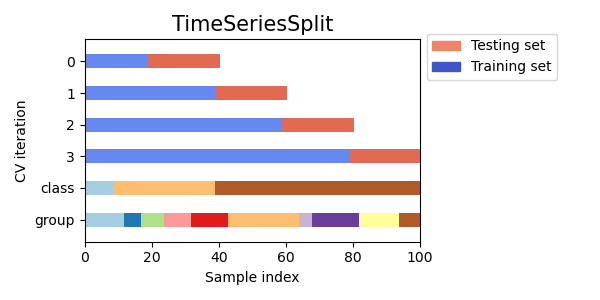
The correct approach is to use a validation strategy that respects the arrow of time. The most common method is rolling-origin cross-validation (also called walk-forward validation or time series cross-validation). In this scheme, the training set grows, and the test set is always chronologically after the training set.
This video provides an excellent visual demonstration of the problem and the solution.
Cross-Validation for Time Series Forecasting | Python Tutorial
This tutorial by Egor Howell clearly illustrates why standard k-fold CV fails for time series and how to implement the correct approach.
Watch the following segments: Standard cross-validation: A quick refresher on k-fold CV in a non-temporal context. Why it fails for time series: This is the core of the problem, explaining data leakage. The correct approach: An introduction to rolling-origin validation.
The scikit-learn library has a specific tool for this, TimeSeriesSplit, which implements this logic. The visualization below shows exactly how it works. In each split, the training set (blue) comes before the testing set (orange), and both move forward in time.
2. Re-framing the Problem for ML Models
Most standard machine learning models, like gradient boosting or simple neural networks, do not have a built-in understanding of sequence or time. If you feed a LightGBM model a sequence of sales numbers, it will treat each number as an independent observation. It has no inherent mechanism to understand the autocorrelation we discussed.
So, how do we use these powerful models for forecasting? We must manually expose the temporal dependencies to the model by transforming the data. This is done by reframing the forecasting problem as a standard supervised learning problem.
The most common technique is the sliding window method. We use past values of the series (lags) as input features (X) to predict a future value (y).
For example, to predict sales at time , we might use sales from , , and as our features.
X = [sales(t-3), sales(t-2), sales(t-1)]y = sales(t)
By doing this, we explicitly encode the temporal relationship in the feature set, allowing any standard supervised learning algorithm to be applied. The following article provides an excellent guide on this concept, which will be a cornerstone of your work when applying ML to forecasting.
Time Series Forecasting as Supervised Learning - MachineLearningMastery.com
This classic article from Machine Learning Mastery explains how to restructure time series data for use with standard ML algorithms. It's a key translational concept for moving from classification to forecasting.
Please read the following sections: Start with the section Sliding Window For Time Series Data. This introduces the core concept with a simple example. Then, read the short comment exchange in the comments section. This directly addresses why preserving order matters and re-confirms the issue with k-fold cross-validation. It's a practical discussion that reinforces what we've learned.
Conclusion
In this lesson, we have laid the critical groundwork for your study of demand forecasting. We've established the fundamental distinction between the i.i.d. world of cross-sectional data you're familiar with and the temporally dependent world of time series.
Here are the key takeaways:
- Cross-sectional data assumes observations are independent and identically distributed (i.i.d.). The order of data does not matter.
- Time series data violates the i.i.d. assumption due to autocorrelation, where observations are dependent on past values.
- This violation has major practical consequences. Standard k-fold cross-validation is invalid as it can lead to data leakage by training on future data to predict the past.
- To evaluate forecasting models, you must use time-aware methods like rolling-origin (or walk-forward) validation.
- To use standard ML algorithms for forecasting, you must reframe the problem into a supervised learning format, typically using a sliding window to create lagged features that explicitly represent the temporal dependencies.
We've focused today on what makes time series special. In our next lesson, we will begin to explore how to analyze the structure within a time series. We will learn to decompose a series into its constituent parts—trend, seasonality, and residuals—which is the first analytical step toward building a robust forecasting model.