Understanding Stationarity in Time Series Analysis

What is Stationarity? An Intuitive View

At its core, a stationary time series is one whose statistical properties—such as the mean, variance, and autocorrelation—are all constant over time. Think of it as a process that is in a state of statistical equilibrium. The distribution from which the observations are drawn does not change.

This might sound abstract, so let's start with a visual and intuitive explanation. The following video introduces the three main criteria for stationarity in a very accessible way.

The examples in the video are excellent for building intuition. Let's connect them to the concepts from our last lesson and the image below.

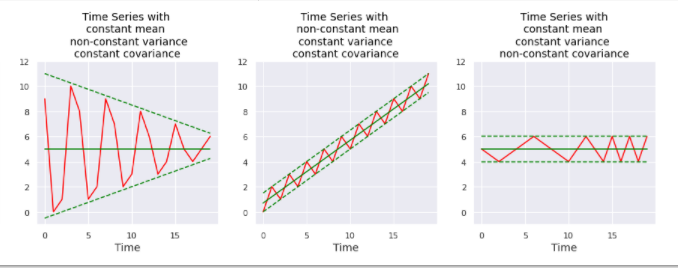
1. Non-constant Mean: The middle plot shows a clear upward trend. The mean of the series in the first half is much lower than the mean in the second half. This is a classic example of non-stationarity. In demand forecasting, this could represent a product with growing popularity.
2. Non-constant Variance: The plot on the left shows a series where the fluctuations are initially large and then dampen over time. This property, where the volatility changes, is called heteroscedasticity and is another form of non-stationarity.
3. Non-constant Covariance/Seasonality: The plot on the right exhibits a clear, repeating pattern. This is a seasonal pattern. Why does this violate stationarity? Because the relationship (covariance) between observations depends on when they occur. For example, the covariance between an observation in a peak month and the next observation will be systematically different from the covariance between an observation in a trough month and the next. The structure of the dependence changes with the season.

A stationary series, by contrast, would look "flat" on average, with constant "width" of fluctuations, and no predictable, repeating patterns. The ritvikmath video also makes a good point distinguishing stationarity from white noise. A white noise process is always stationary, but a stationary process is not necessarily white noise, as it can still have autocorrelation (as long as that autocorrelation structure is constant over time).

Formalizing Stationarity: Weak vs. Strict

The intuitive definition is a great start, but in practice, we need more precise, mathematical definitions. This leads to a crucial distinction between two types of stationarity: strong (or strict) and weak (or covariance).

The next video clearly explains this distinction.

As you saw, strong stationarity is a very restrictive condition. It requires the entire probability distribution—including all its moments (mean, variance, skewness, kurtosis, etc.)—to remain identical through time. While this is theoretically clean, it's rarely met by real-world data, especially in economics and commerce.

This is why, for most practical applications, we rely on weak stationarity. The conditions for weak stationarity are precisely the ones we discussed intuitively, but stated mathematically:

A time series $Y_t$ is weakly stationary if it satisfies three conditions:

1. The mean is constant: $$E[Y_t]=\mu \text{for all }t$$
2. The variance is constant: $$Var(Y_t)=E[(Y_t-\mu {)}^2]={\sigma }^2\text{for all }t$$
3. The autocovariance depends only on the lag: $$Cov(Y_t,Y_{t-k})=E[(Y_t-\mu )(Y_{t-k}-\mu )]=\gamma (k)\text{for all }t,k$$

The third condition is the most subtle. It says the covariance between two points only depends on how far apart they are in time (the lag $k$), not on where they are in the series (the time $t$). This is the condition that seasonality violates.

For a deeper look at these formal definitions, you can consult the following resource.

From here on, unless specified otherwise, "stationarity" will refer to weak stationarity, as it is the standard for building classical time series models.

Why Does Stationarity Matter?

Now for the crucial question: why do we care so much about this property? Why do models like ARIMA assume it?

The fundamental reason is learnability and predictability. Classical forecasting models work by learning the statistical properties of a time series from past data. They estimate a mean, a variance, and an autocorrelation structure. The central assumption is that these learned properties will remain the same in the future. The model then uses these stable properties to make predictions.

If the series is non-stationary, this core assumption is broken.

• If there's a trend (non-constant mean), what is the "mean" of the series? It's changing. The average value from the first half of your data is a poor estimate for the average value in the future.
• If the variance is changing, a model might predict a range of future values that is far too narrow or wide.
• If the covariance structure changes, the way past values relate to future values is not stable, making historical correlations a misleading guide.

Let's illustrate with a classic non-stationary process: the random walk. A random walk with drift is defined as $y_t=\mu +y_{t-1}+{ϵ}_t$, where ${ϵ}_t$ is white noise. This model essentially says that the value at time $t$ is the previous value plus a constant drift and a random shock. Stock prices and other financial series are often modeled this way.

The lecture notes you just consulted show precisely why this process is non-stationary.

As the derivation shows, both the mean ($E[y_t]=\mu t+y_0$) and the variance ($Var[y_t]={\sigma }^{2}t$) depend explicitly on time $t$. They are not constant. A model that assumes a constant mean would fail to capture the behavior of a random walk. This is why models that contain a "unit root" (like a random walk where the coefficient on $y_{t-1}$ is 1) are non-stationary and require special handling.

This is the primary motivation for the techniques we will learn in upcoming lessons. We will need to:

1. Test for stationarity to see if a problem exists.
2. Transform non-stationary data to make it stationary before we can apply models like ARIMA. The decomposition you performed in the last lesson is a first step—by isolating and removing the trend and seasonal components, you are in effect trying to produce a stationary residual series.

Conclusion

In this lesson, we have formally defined stationarity and explored its critical importance for time series modeling. This concept acts as a bridge between observing the structure of a time series and formally modeling it.

Here are the key takeaways:

• A stationary process has statistical properties (mean, variance, covariance structure) that do not change over time.
• Strict stationarity requires the entire joint probability distribution to be time-invariant, a condition rarely met in practice.
• Weak stationarity is a more practical definition, requiring only the mean, variance, and autocovariance to be constant. This is the standard assumption for many classical models.
• Stationarity is crucial because it ensures that the patterns learned from the past are a reliable guide for the future. Models like ARIMA depend on this stability to make predictions.
• Common sources of non-stationarity, such as trends and seasonality, must be identified and handled before applying these models.

You now understand what stationarity is and why it's so important. The natural next question is, "How do I know if my data is stationary?" In our next lesson, we will answer exactly that. We will move from visual inspection to formal statistical procedures, learning how to use the Augmented Dickey-Fuller (ADF) and KPSS tests to rigorously check for stationarity in your data.