Hello! Welcome back to your course on diffusion models.
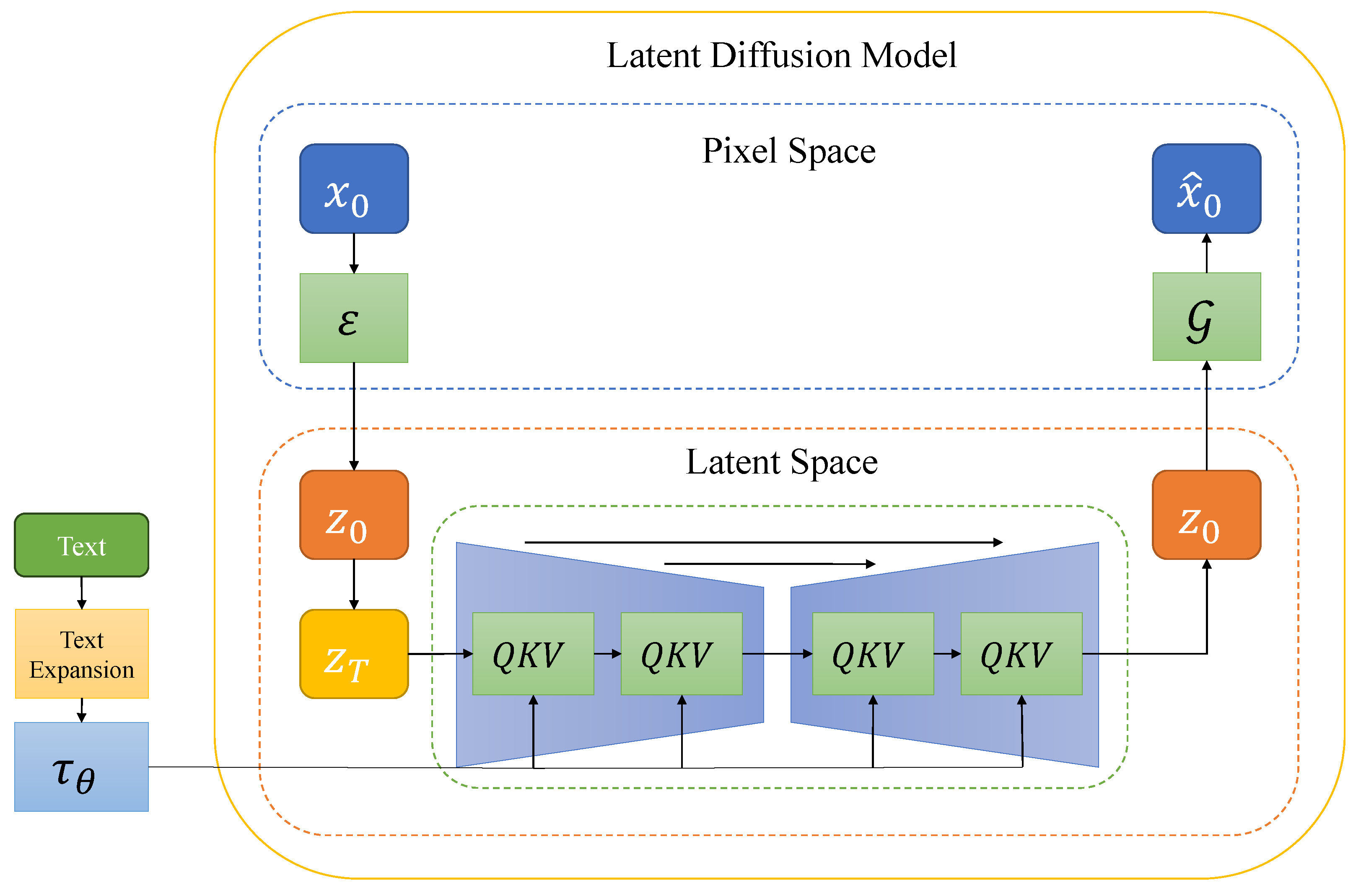
In our last two lessons, we built the core components of a Latent Diffusion Model (LDM). First, we trained a high-fidelity Variational Autoencoder (VAE) to compress images. Then, we adapted a DDPM-style training loop to run the diffusion process entirely within the VAE's compact latent space. This two-stage approach adds complexity compared to a simple pixel-space DDPM.
Today's lesson addresses the crucial question: Why bother? Our learning outcome is to compare the computational efficiency and generation quality of pixel-space vs. latent-space diffusion. We'll move from "how" to "why," analyzing the concrete trade-offs and quantifying the benefits that have made LDMs the dominant architecture for image generation.
The Problem with Pixels: A Costly Playground
Diffusion models that operate directly on pixels are powerful, but they come with a significant computational burden. The U-Net, the workhorse of the model, must process a high-dimensional tensor at every single step of the diffusion process. For a 256x256 RGB image, that's a tensor with 196,608 values. This has major consequences:
- Training is slow and expensive: Backpropagating through the U-Net for hundreds of thousands of steps on large tensors consumes immense GPU time and memory.
- Inference is slow: Generating a single image requires hundreds of sequential forward passes through this large network.
Furthermore, as you've seen with VAEs, much of the information in an image (e.g., fine-grained texture, high-frequency noise) is perceptually insignificant. A pixel-space model wastes a substantial portion of its capacity learning to model these minute details, which could be better spent on capturing the core semantic content.
The video below offers a great summary of these limitations, motivating the need for a more efficient approach.
Stable Diffusion from Scratch in PyTorch | Unconditional Latent Diffusion Models
The 'ExplainingAI' channel provides a concise overview of the computational challenges that pixel-space diffusion models face, especially as image resolution and dataset complexity increase.
Watch from 03:21 to 04:45. The video quantifies the training cost of early pixel-space models, highlighting why a new approach was necessary to make high-resolution training feasible on reasonable hardware.
This challenge is precisely what latent diffusion was designed to solve. By moving the expensive iterative process into a smaller, compressed space, we aim to improve efficiency without sacrificing—and perhaps even improving—quality.
Axis 1: Computational Efficiency
The most direct benefit of latent diffusion is the dramatic improvement in computational efficiency across the board.
Training and Inference Speed
By performing diffusion on a compressed latent representation, we drastically reduce the size of the tensors the U-Net has to process. Consider the example from the High-Resolution Image Synthesis With Latent Diffusion Models paper (often called the LDM or Stable Diffusion paper). A 256x256x3 image is compressed into a 32x32x4 latent space.
- Pixel-space tensor size: values
- Latent-space tensor size: values
This represents a 48x reduction in the number of elements the U-Net processes at each step. This directly translates to faster training iterations and faster sampling steps. The only added costs are a single forward pass through the encoder during data preparation and a single forward pass through the decoder at the end of sampling, which are negligible compared to the hundreds of iterative diffusion steps.
The original LDM paper provides clear empirical evidence for this.
High-Resolution Image Synthesis With Latent Diffusion Models
The foundational LDM paper by Rombach et al. includes a section dedicated to analyzing these performance trade-offs. We'll focus on the figures and tables that directly compare pixel-space and latent-space models.
Please study Section 4.1, 'On Perceptual Compression Tradeoffs'. Figure 5 is key. It plots sample quality (FID) against training steps. Notice how LDM-1 (pixel-based) trains much slower than the latent models (LDM-4, LDM-8). Figure 6 compares inference speed vs. quality. Observe the dramatic difference in samples/second between LDM-1 and the latent models. Table 6 provides a direct throughput comparison for an inpainting task. Compare the hours/epoch for LDM-1 vs. LDM-4. This quantifies the training speed-up.
As the paper demonstrates, LDM-4 achieves a training speed-up of approximately 2.7x over a pixel-based model (LDM-1), while inference throughput can be orders of magnitude higher for a comparable quality level.
Memory Footprint
Reduced tensor sizes also lead to a smaller memory footprint. The activations stored during the forward pass are much smaller, which means less VRAM is needed for the backward pass during training. This has practical benefits:
- It allows for larger batch sizes, which can stabilize and accelerate training.
- It makes it possible to train and run powerful models on consumer-grade GPUs, democratizing access to this technology.
This point is well-articulated in the following blog post, which provides a superb high-level overview of the move to latent space.
Generative modelling in latent space
Sander Dieleman's blog post 'Generative modelling in latent space' offers a clear, conceptual explanation of why the two-stage approach is so effective.
Read the subsection 'Latent diffusion' and the section that follows, 'Why two stages?'. Focus on the two reasons provided for why the two-stage approach is complementary to the perceptual nature of the diffusion loss itself. The second point directly addresses the computational benefits, including reduced memory requirements and faster training/sampling.
Axis 2: Generation Quality
Efficiency gains are meaningless if the final images are poor. One might intuitively expect that compressing an image into a latent space—a "lossy" process—would inevitably degrade the maximum achievable quality. However, the opposite is often true.
The Importance of a High-Fidelity Autoencoder
The quality of an LDM is fundamentally capped by the reconstruction quality of its VAE. If the VAE produces blurry outputs, the LDM can't magically invent the lost detail. This is why, as we saw in a previous lesson, training the VAE is so critical. A simple L2 (MSE) reconstruction loss is insufficient because it averages over many possible high-frequency details, leading to blurriness.
To achieve sharp, realistic reconstructions, the VAE is trained with a composite loss function:
- Reconstruction Loss (e.g., L1): Ensures the output is structurally similar to the input.
- Perceptual Loss (e.g., LPIPS): Uses a pre-trained network (like VGG) to enforce similarity in feature space, which correlates better with human perception and preserves textures.
- Adversarial Loss (GAN Loss): A discriminator network pushes the decoder to produce outputs that are indistinguishable from real images, enforcing realism and high-frequency detail.
This combination ensures the latent space retains all the perceptually relevant information needed for high-quality generation.
Stable Diffusion from Scratch in PyTorch | Unconditional Latent Diffusion Models
Let's revisit the 'ExplainingAI' video, which does an excellent job of breaking down why this multi-part loss is essential for quality.
Watch the segment from 07:31 to 19:32. It covers, in sequence: Why simple reconstruction loss leads to blurry images (07:31). How perceptual loss (LPIPS) solves this by comparing images in a learned feature space (08:37). How adversarial loss adds the final layer of realism by training the decoder to 'fool' a discriminator (16:29).
Can Latent Models Surpass Pixel-Space Quality?
With a high-quality VAE, LDMs can indeed achieve superior results to their pixel-space counterparts. The key insight is that by delegating the task of modeling fine-grained, perceptually irrelevant noise to the VAE, the diffusion model can focus its entire capacity on the more important task: learning the semantic and conceptual composition of the data.
The model is no longer wasting resources trying to get every single pixel perfect in a noisy texture; instead, it's learning the relationship between "cat," "sofa," and "sunbeam."
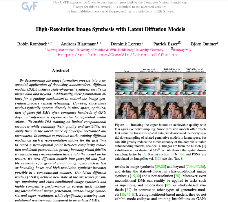
The empirical results from the LDM paper confirm this. Look again at Figure 5 from the High-Resolution Image Synthesis... paper (LINK). Not only do the latent models (LDM-4, LDM-8) train faster, but their final FID scores are significantly lower (better) than the pixel-based LDM-1. This demonstrates that the two-stage approach provides both an efficiency and a quality advantage.
Test your understanding!
You are tasked with designing a latent diffusion model for generating high-resolution medical images (e.g., 1024x1024 MRIs). You are considering two VAEs for the first stage:
- VAE A: Has a large downsampling factor (e.g.,
f=32), resulting in a very small latent space. It's extremely fast to train a diffusion model on top of it. - VAE B: Has a moderate downsampling factor (e.g.,
f=8), resulting in a larger latent space. Training the diffusion model is slower than with VAE A, but still much faster than a pixel-space model.
In medical imaging, preserving fine details like small lesions or tissue boundaries is critical. Which VAE is the more appropriate choice, and why? What is the primary risk associated with the other choice?
Show answer
VAE B is the more appropriate choice.
Here's why:
- Quality over Speed: For medical imaging, diagnostic quality is paramount. A moderate downsampling factor (
f=8) strikes a better balance, ensuring that critical high-frequency details (lesions, boundaries) are preserved in the latent space. - Risk of VAE A: The primary risk of VAE A (
f=32) is information loss. The aggressive compression might discard the very details that are diagnostically important. No matter how powerful the subsequent diffusion model is, it cannot generate details that were completely erased by the VAE's encoder. The final image quality would be fundamentally capped by the VAE's poor reconstruction fidelity for fine structures.
This highlights the critical trade-off: the VAE's compression factor must be chosen carefully to balance computational efficiency with the information preservation required for the specific task.
Conclusion: The Best of Both Worlds
Today, we've dissected the "why" behind latent diffusion. By moving from pixel space to a compressed latent space, we don't just make things faster; we create a more effective division of labor that can lead to better results.
Key Takeaways:
- Computational Efficiency: Latent diffusion is significantly faster in training and inference and requires less memory than pixel-space diffusion. This is due to the U-Net operating on a much smaller tensor representation.
- Generation Quality: By using a high-fidelity VAE (trained with perceptual and adversarial losses), LDMs can achieve superior generation quality. The diffusion model focuses its capacity on semantic content rather than imperceptible noise.
- The Compression Trade-off: The choice of the VAE's downsampling factor is a critical design decision. Too much compression leads to information loss and limits quality. Too little compression reduces the efficiency gains. The optimal point balances these two concerns.
- A New Paradigm: The two-stage approach has proven so effective that it has become the standard for most state-of-the-art image and video generation models, even though it adds engineering complexity.
Next Lesson Preview:
So far, our focus has been on the model architectures and training processes. In the next module, we will shift our attention entirely to inference and sampling. Our first lesson will cover how to "Implement ancestral sampling with different noise schedules." We'll explore how the schedule of noise levels used during the reverse process affects generation speed and quality, giving you another lever to control the trade-offs in your diffusion models.