Training Latent Diffusion Models

1. The Full Picture: Diffusion in Latent Space

Let's start with a high-level overview. The entire process now consists of two distinct, sequential stages:

1. Perceptual Compression (VAE): An image is passed through the VAE's encoder to get a compressed latent vector. This is a one-time, feed-forward step.
2. Latent Diffusion (U-Net): The diffusion process (both forward noising during training and reverse denoising during sampling) happens entirely in the latent space.
3. Image Generation (VAE): Once the U-Net has produced a "clean" latent vector, it's passed through the VAE's decoder to generate the final, full-resolution image.

The diagram below perfectly illustrates this workflow. The VAE encoder and decoder act as portals between the pixel world and the latent world, where the U-Net operates.

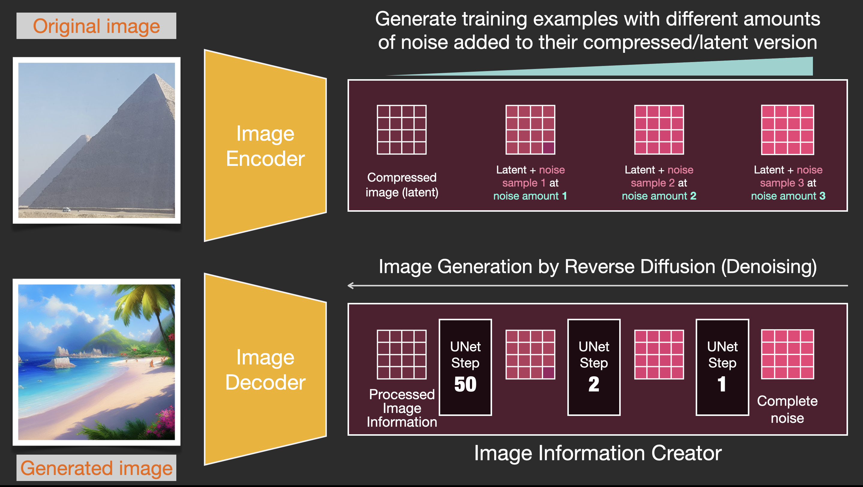
Your previous experience implementing a DDPM in pixel space is the perfect foundation. Today, we're essentially modifying that existing recipe to work on latents instead of pixels.

2. Adapting the Data Pipeline: From Pixels to Latents

The most significant change is in how we handle our data. In a standard DDPM, the training loop consumes batches of images. In a Latent Diffusion Model (LDM), the training loop consumes batches of latent vectors.

A naive approach would be to encode images to latents on-the-fly inside the training loop. However, since the VAE is frozen, this encoding step is deterministic and computationally redundant. A much more efficient strategy, especially for large datasets, is to pre-process the entire dataset.

This involves a one-time pass where you:

1. Load every image from your original dataset.
2. Pass it through the trained VAE's encoder.
3. Save the resulting latent vector.
4. Create a new dataset composed entirely of these latent vectors.

Your diffusion model's training loop then loads data directly from this new, pre-computed latent dataset.

3. Adapting the Training Loop

With our latent dataset ready, let's adapt the training loop. The core logic of diffusion—adding noise and training a model to predict it—remains identical. The only thing that changes is the domain in which it operates.

The video below provides a fantastic, concise walkthrough of the necessary code modifications. It starts with a standard DDPM training script and shows the exact lines that need to be changed to convert it into an LDM.

Let's solidify this with a step-by-step breakdown of the training code. The overall structure will look very familiar.

1. Load Models:

   • Load your pre-trained VAE and freeze its parameters (vae.eval() and for param in vae.parameters(): param.requires_grad = False).
   • Instantiate your U-Net. Crucially, the in_channels and out_channels must now match the channel dimension of your VAE's latent space (e.g., 4 or 32, not 3 for RGB).

2. The Training Step: For each batch from your latent dataset:

   • You receive a batch of clean latent vectors, latents.
   • Scaling: It's common practice to scale the latents by a constant factor before adding noise. This helps match the variance of the latents to the expected input variance of the U-Net (often near unit variance).
   • Forward Diffusion:
     • Sample random timesteps t.
     • Sample random noise noise from a standard normal distribution, with the same shape as latents.
     • Create noisy latents: noisy_latents = scheduler.add_noise(latents, noise, t).
   • Noise Prediction: Pass the noisy_latents and t through the U-Net to get predicted_noise.
   • Loss Calculation: Compute the loss, typically MSE, between the predicted_noise and the original noise.
     loss = F.mse_loss(predicted_noise, noise)
   • Backpropagation: loss.backward() and optimizer.step() to update the U-Net's weights. The VAE weights remain frozen.

The following reading provides a complete, runnable code example that puts all these pieces together.

# Simplified DDPM training step
def train_step(images, unet_model, scheduler, optimizer):
    # images shape: [batch_size, 3, 64, 64]
    
    # 1. Sample timesteps
    t = torch.randint(0, scheduler.num_timesteps, (images.shape[0],), device=images.device)
    
    # 2. Create noisy images (forward process)
    noise = torch.randn_like(images)
    noisy_images = scheduler.add_noise(images, noise, t)
    
    # 3. Predict noise with U-Net
    predicted_noise = unet_model(noisy_images, t)
    
    # 4. Calculate loss
    loss = F.mse_loss(predicted_noise, noise)
    
    # 5. Backpropagate
    optimizer.zero_grad()
    loss.backward()
    optimizer.step()
    
    return loss

# Adapted LDM training step
def train_step_ldm(images, vae_model, scaling_factor, unet_model, scheduler, optimizer):
    # images shape: [batch_size, 3, 64, 64]
    
    # CHANGE 1: Encode images into latents and disable VAE gradients
    with torch.no_grad():
        latents = vae_model.encode(images).latent_dist.sample() * scaling_factor
    # latents shape is now something like: [batch_size, 4, 8, 8]
    
    # 1. Sample timesteps
    t = torch.randint(0, scheduler.num_timesteps, (latents.shape[0],), device=latents.device)
    
    # CHANGE 2: Create noisy LATENTS, not images
    noise = torch.randn_like(latents)
    noisy_latents = scheduler.add_noise(latents, noise, t)
    
    # 3. Predict noise with U-Net from noisy LATENTS
    predicted_noise = unet_model(noisy_latents, t)
    
    # CHANGE 3: Calculate loss against the latent noise
    loss = F.mse_loss(predicted_noise, noise)
    
    # 5. Backpropagate (only updates unet_model)
    optimizer.zero_grad()
    loss.backward()
    optimizer.step()
    
    return loss

4. Adapting the Inference/Sampling Loop

The adaptation for inference mirrors the training loop. You start with a random tensor in the latent space and use the U-Net to iteratively denoise it.

The key difference is the very last step: once the scheduler has produced the final "clean" latent vector latent_0, you must pass it through the VAE's decoder to get the final pixel-space image.

final_image = vae_model.decode(latent_0 / scaling_factor).sample

Note the division by the scaling_factor to reverse the scaling operation we applied during training.

Conclusion

In this lesson, we completed the second stage of our two-stage model. By adapting the familiar DDPM training process to operate in a compressed latent space, we've built a full Latent Diffusion Model.

Key Takeaways:

• Two-Stage Process: LDMs separate perceptual compression (VAE) from the generative diffusion process (U-Net).
• Frozen VAE: During diffusion training, the pre-trained VAE is frozen and used solely to convert images to latents. Its weights are not updated.
• Latent Space Operations: The entire diffusion process—adding noise, U-Net prediction, and calculating loss—occurs on latent vectors, not pixels.
• Adaptations: The primary code changes involve:
  1. A data preprocessing step to encode images into a latent dataset.
  2. Modifying the U-Net's channel configuration to match the latent dimension.
  3. A final decoding step during inference to convert the generated latent back into an image.

Next Lesson Preview:

We've now seen how to build both a pixel-space DDPM and a latent-space LDM. But was the added complexity of the LDM worth it? In the next lesson, we will compare the computational efficiency and generation quality of pixel-space vs. latent-space diffusion. We'll conduct practical experiments to quantify the trade-offs in terms of training time, memory usage, and the quality of the final generated images, solidifying the motivation behind this powerful architectural shift.