Quantization and Mixed-Precision for Optimized Inference

1. The Need for Speed (and Less Memory)

Diffusion models, especially large ones for high-resolution image or video generation, come with significant computational baggage:

• Memory Footprint: A model like FLUX.1-dev requires over 30GB of VRAM just to load in its standard bfloat16 precision. This limits the hardware it can run on and increases deployment costs.
• Inference Latency: The iterative denoising process, often involving 20-50 full model passes, makes generation slow. For interactive applications or large-scale asset production, this latency is a major bottleneck.

To tackle these issues, we'll explore two powerful techniques: quantization and mixed precision.

2. Quantization: Doing More with Less

Quantization is the process of reducing the numerical precision of a model's parameters (weights) and, in some cases, its activations. The most common approach is to convert 32-bit floating-point numbers (FP32) into 8-bit integers (INT8).

This has two primary benefits:

1. Reduced Memory: Storing a weight as an INT8 value requires 4x less memory than FP32.
2. Faster Computation: Integer arithmetic is significantly faster than floating-point arithmetic on most modern hardware, especially on specialized cores like NVIDIA's Tensor Cores.

To understand the fundamentals of how this works, the following video provides an excellent and comprehensive explanation.

Key Quantization Concepts

As you saw in the video, quantization isn't just round(x). It's a mapping that preserves the relative distribution of the original floating-point values within a smaller integer range.

• Asymmetric Quantization: Maps the exact range [min_float, max_float] to [min_int, max_int]. The floating-point zero may not map to an integer zero. This is flexible but can require more complex calculations due to the zero-point offset.
• Symmetric Quantization: Maps a symmetric range [-abs_max_float, +abs_max_float] to a symmetric integer range [-max_int, +max_int]. This ensures that the floating-point zero always maps to the integer zero, simplifying computation.

Post-Training Quantization (PTQ)

For optimizing inference, Post-Training Quantization (PTQ) is the most common approach. We take a fully trained FP32 or FP16 model and convert its weights to a lower precision like INT8.

The process involves:

1. Calibration: We run a small, representative sample of data through the model to observe the dynamic range (min and max values) of the weights and, crucially, the activations at each layer.
2. Quantization: Using these observed ranges, we calculate the scale and zero-point for each layer and convert the weights to INT8. The model is now ready for fast integer-based inference.

The video you watched demonstrates this process with PyTorch, highlighting how observers are used to collect statistics for calibration.

While PTQ is fast and doesn't require retraining, it can sometimes lead to a drop in accuracy. If the accuracy loss is too severe, an alternative is Quantization-Aware Training (QAT), which simulates the effects of quantization during the training process, allowing the model to adapt and become more robust to precision loss. This typically yields better accuracy than PTQ but requires a full training or fine-tuning run.

3. Mixed Precision: The Best of Both Worlds

Mixed precision is a technique, primarily used during training but also relevant for inference, that combines different floating-point precisions to balance speed, memory, and numerical stability.

The standard approach uses:

• FP16 (Half Precision): For the bulk of the computations (matrix multiplications in forward and backward passes). This halves the memory usage compared to FP32 and leverages hardware acceleration.
• FP32 (Single Precision): For critical parts where precision is paramount, like accumulating gradients and updating the master copy of the weights.

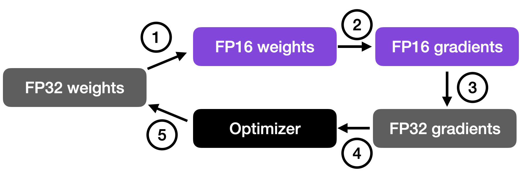
Two key components make this work: a master copy of the weights and loss scaling.

Modern diffusion models are typically trained using BF16 or FP16 from the start. For inference, you often load the model in this native precision. Further optimization then comes from applying quantization on top of this.

4. Practical Application: Quantizing a Diffusion Model

Now, let's apply these concepts to a real diffusion model. The Hugging Face diffusers library provides a streamlined way to load models with various quantization backends. We will focus on bitsandbytes, a popular library for 8-bit and 4-bit quantization.

Let's break down the key implementation pattern from the article.

import torch
from diffusers import FluxPipeline
# Import the specific config classes for the backend you are using
from diffusers import BitsAndBytesConfig as DiffusersBitsAndBytesConfig
from diffusers.quantizers import PipelineQuantizationConfig
from transformers import BitsAndBytesConfig as TransformersBitsAndBytesConfig

model_id = "black-forest-labs/FLUX.1-dev"

# 1. Define the quantization configuration for the pipeline
pipeline_quant_config = PipelineQuantizationConfig(
    # A mapping from model component name to its quantization config
    quant_mapping={
        # Quantize the main diffusion transformer
        "transformer": DiffusersBitsAndBytesConfig(
            load_in_4bit=True, 
            bnb_4bit_quant_type="nf4", # NormalFloat 4-bit is often best for quality
            bnb_4bit_compute_dtype=torch.bfloat16
        ),
        # Also quantize the large T5 text encoder
        "text_encoder_2": TransformersBitsAndBytesConfig(
            load_in_4bit=True, 
            bnb_4bit_quant_type="nf4", 
            bnb_4bit_compute_dtype=torch.bfloat16
        ),
    }
)

# 2. Load the pipeline with the quantization config
pipe = FluxPipeline.from_pretrained(
    model_id,
    quantization_config=pipeline_quant_config,
    torch_dtype=torch.bfloat16 # Compute dtype should match
)
pipe.to("cuda")

# Now the pipeline is ready for inference with significantly less VRAM usage.

As the benchmark table in the article shows, using 4-bit quantization with bitsandbytes reduces the peak memory usage for the FLUX model from ~36 GB down to ~17 GB—a massive saving that makes the model accessible on a much wider range of GPUs. Notice that for bitsandbytes, the inference time isn't necessarily faster without further optimization like torch.compile. The primary benefit here is the memory reduction.

The Frontier: FP8 Quantization

While INT8 and INT4 are powerful, the latest hardware, like NVIDIA's Hopper architecture, introduces native support for FP8 (8-bit floating-point) precision. This offers a compelling alternative to integer quantization.

FP8 comes in two main flavors:

• E4M3 (4 exponent bits, 3 mantissa bits): More precision, smaller dynamic range. Better for inference where value distributions are often stable.
• E5M2 (5 exponent bits, 2 mantissa bits): Less precision, wider dynamic range. Better for training where gradients can have large spikes.

Industry leaders are already leveraging this. For example, Adobe used FP8 with NVIDIA's TensorRT to optimize their Firefly video generation model, achieving a 60% reduction in latency.

The diffusers blog post also mentions backends like torchao and Quanto which are beginning to support these newer FP8 data types, showing that the ecosystem is rapidly evolving towards more efficient formats.

Conclusion

In this lesson, we've taken our first major step into the world of model optimization. You now have the foundational knowledge to make large, cumbersome diffusion models practical for deployment.

Key Takeaways:

• Quantization drastically reduces memory footprint and can accelerate inference by converting high-precision floating-point weights to low-bit integers (e.g., INT8, INT4).
• Mixed Precision (e.g., FP16/BF16 with FP32 master weights) is a standard technique for efficient training and a common starting point for inference optimization.
• Post-Training Quantization (PTQ) is a practical method for optimizing pre-trained models for inference, often involving a calibration step to determine value ranges.
• Modern libraries like diffusers and bitsandbytes make it straightforward to apply these techniques, often with just a few lines of configuration code.
• The field is constantly evolving, with newer formats like FP8 offering even better performance on the latest hardware.

Next Lesson Preview:

Quantization is just one tool in our optimization toolbox. Another powerful technique is to train a smaller, faster "student" model to mimic the behavior of a large, slow "teacher" model. In the next lesson, we will explore this concept by learning how to implement progressive distillation to train a faster student model from a multi-step teacher.