Sinusoidal Positional Encodings for U-Net Timestep Conditioning

1. Why Does the U-Net Need Timestep Information?

The core of a diffusion model is a single neural network (our U-Net) that is used at every step of the reverse process. This means the same set of weights is responsible for predicting the noise in a slightly noisy image (e.g., at $t=50$) and a nearly pure-noise image (e.g., at $t=950$).

The network must adapt its behavior based on the noise level. A raw integer timestep t is not an ideal input for a neural network. Neural networks thrive on continuous, high-dimensional inputs where small changes in input correspond to small changes in output. A simple integer doesn't have this property in a way the network can easily leverage. The difference between t=1 and t=2 is not necessarily the same "semantic distance" as between t=901 and t=902. We need a more powerful way to encode this positional information.

2. Sinusoidal Positional Encodings

As the video mentioned, the solution comes from the original Transformer paper ("Attention Is All You Need"). We can map the scalar integer timestep $t$ into a high-dimensional vector using a set of sine and cosine functions of varying frequencies.

The formula for an embedding of dimension $d$ for a timestep $t$ is:

where $i$ indexes the dimensions of the embedding vector from $0$ to $d/2-1$.

This method has several desirable properties:

• Uniqueness: Every timestep gets a unique encoding vector.
• Continuity: For nearby timesteps $t_1$ and $t_2$, their embeddings $PE(t_1)$ and $PE(t_2)$ will be close in Euclidean space, making it easier for the network to generalize.
• Extrapolation: The periodic nature of sine and cosine allows the model to potentially generalize to timesteps longer than those seen during training.

The result is a rich, high-dimensional representation of time. Let's visualize what these embeddings look like.

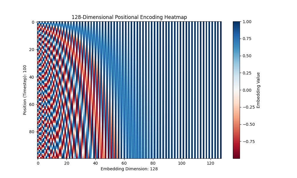
3. Implementation in PyTorch

Now, let's translate the theory into a practical PyTorch module. The Hugging Face blog post "The Annotated Diffusion Model" provides a very clean and standard implementation.

Let's break down the forward method of this module. It's a clever and efficient way to implement the formulas above:

1. half_dim = self.dim // 2: We calculate separate sine and cosine components for each half of the embedding dimension.
2. embeddings = math.log(10000) / (half_dim - 1): This calculates the logarithmic term from the denominator of the formula.
3. embeddings = torch.exp(torch.arange(half_dim, device=device) * -embeddings): This creates the vector of different frequencies/wavelengths (1 / 10000^(2i/d)).
4. embeddings = time[:, None] * embeddings[None, :]: This uses broadcasting to apply all frequencies to all timesteps in the batch simultaneously, calculating the argument for the sine and cosine functions.
5. embeddings = torch.cat((embeddings.sin(), embeddings.cos()), dim=-1): Finally, it computes the sine and cosine and concatenates them to form the final embedding vectors.

4. Integrating Embeddings into the U-Net

Now that we have a time embedding vector for each image in our batch, how do we use it? We need to inject this information into the U-Net's processing pipeline.

The standard approach involves two steps:

1. Projection: The sinusoidal embedding is first passed through a small Multi-Layer Perceptron (MLP), typically Linear -> Activation -> Linear. This allows the model to learn a more suitable representation of the time information.
2. Injection: This learned time embedding is then broadcast and added to the intermediate feature maps inside the U-Net. This is usually done within each residual block of the U-Net's encoder and decoder.

The diagram below gives a high-level view of how the time embedding is incorporated into a residual block.

Let's watch a short video that walks through the code for this integration process.

An Alternative: Feature-wise Linear Modulation (FiLM)

While simple addition is common, a more powerful technique is to use the time embedding to generate scale and shift parameters that modulate the feature maps. This is a form of FiLM (Feature-wise Linear Modulation).

Instead of h_out = h_in + time_emb, we do h_out = h_in * scale + shift.

The scale and shift are produced by the time embedding MLP. This gives the time conditioning more expressive power, as it can dynamically scale and shift activations at each block, rather than just adding a bias.

The ResnetBlock implementation in "The Annotated Diffusion Model" uses exactly this more advanced technique.

import torch
import torch.nn as nn

# Assuming these are defined elsewhere
# t_emb = sinusoidal_embedding_module(timesteps) -> shape [16, 128]
# x = some_conv_layer(input) -> shape [16, 256, 32, 32]

# 1. Define the projection MLP (this would be part of the block's __init__)
time_mlp = nn.Sequential(
    nn.Linear(128, 256),
    nn.ReLU(),
    nn.Linear(256, 256)
)

# 2. Process the time embedding (this happens in the forward pass)
t_emb_projected = time_mlp(t_emb) # shape: [16, 256]

# 3. Reshape for broadcasting and add to the feature map
# Add new dimensions for height and width to match x
t_emb_reshaped = t_emb_projected[:, :, None, None] # shape: [16, 256, 1, 1]
output = x + t_emb_reshaped # Broadcasting adds the embedding to each pixel

# 'output' now has shape [16, 256, 32, 32] and is conditioned on the timestep

Conclusion

In this lesson, we took our first major step inside the U-Net. We've replaced a key "magic" component with a concrete, understandable, and implementable mechanism.

Key Takeaways:

• The U-Net in a diffusion model needs to be conditioned on the timestep t because its weights are shared across the entire denoising trajectory.
• We encode the scalar timestep t into a high-dimensional vector using sinusoidal positional encodings, a technique borrowed from Transformers that provides a unique and continuous representation for each timestep.
• This time embedding vector is first projected through a small MLP.
• The projected embedding is then injected into each residual block of the U-Net, either by direct addition to the feature maps or by generating scale and shift parameters to modulate them (FiLM).

Next Lesson Preview:

Now that we understand how to condition the U-Net on time, we can extend this idea to other forms of conditioning. The U-Net architecture is not just a stack of residual blocks; it crucially relies on attention mechanisms. In our next lesson, we will integrate self-attention and cross-attention mechanisms. Self-attention will help the model capture long-range spatial dependencies within the image, and cross-attention will be our gateway to powerful external conditioning, such as text prompts.