Understanding CNN Architecture and Computer Vision Applications

1. The Problem with Images

Imagine trying to classify a 224x224 pixel color image using the fully-connected network we studied previously. A color image has 3 channels (Red, Green, Blue), so the input size is 224 x 224 x 3 = 150,528 pixels. If we were to flatten this into a single vector and connect it to a hidden layer of, say, 1000 neurons, that single connection would require over 150 million weights. This approach presents two critical problems:

1. Massive Parameter Count: The number of weights would be computationally immense, making the network extremely slow to train and highly prone to overfitting.
2. Loss of Spatial Structure: By flattening the image into a long vector, we destroy the spatial relationships between pixels. The fact that a pixel is above or to the left of another is crucial information for understanding an image, but a fully-connected layer treats all input pixels independently.

To see a more detailed explanation of these challenges, let's watch the beginning of a lecture from MIT's Deep Learning course.

Clearly, a more intelligent approach is needed—one that preserves and leverages the spatial nature of images.

2. The Core Idea: Convolution as Feature Detection

How do humans recognize an object in an image? We don't process every pixel individually. Instead, we identify key features—edges, corners, textures, and shapes. We then recognize that a certain combination of features (e.g., two round shapes above a vertical line) constitutes a more complex object (a face).

CNNs are inspired by this process. They use a mathematical operation called convolution to act as a feature detector. The core components are:

• Filter (or Kernel): A small matrix of weights (e.g., 3x3 or 5x5). Each filter is designed to detect a specific, low-level feature, like a vertical edge or a patch of a certain color.
• Convolution Operation: The filter "slides" across the input image. At each position, the network performs an element-wise multiplication between the filter's weights and the corresponding pixels in the image patch, then sums up the results.
• Feature Map (or Activation Map): The output of this sliding operation is a new 2D matrix called a feature map. High values in the feature map indicate locations where the filter's specific feature was detected in the input image.

This next video provides an excellent, intuitive explanation of how this works.

The crucial insight here is parameter sharing. The same small filter (with the same set of weights) is used across the entire image. This is what makes CNNs so efficient. Instead of learning a separate weight for every pixel, the network only learns the weights for the filters, which then detect features regardless of where they appear in the image. This property is known as translation invariance.

3. The Architecture of a Convolutional Neural Network

A complete CNN is built by stacking several layers. A typical "convolutional block" consists of three stages: convolution, a non-linear activation, and pooling.

3.1. The Convolutional Layer

A single convolutional layer usually applies multiple filters to its input. Each filter learns to detect a different feature. If a layer has 32 filters, it will produce 32 corresponding feature maps. This output is a "volume" of data (width x height x 32).

To see the convolution operation and the idea of learning filters in more detail, let's return to the MIT lecture.

3.2. Activation Function (ReLU)

Just like in standard neural networks, after the linear operation of convolution, we apply a non-linear activation function. In CNNs, the most common choice is the Rectified Linear Unit (ReLU).

$\text{ReLU}(x)=\max (0,x)$

ReLU simply replaces all negative values in the feature map with zero. It's computationally simple and has been shown to work very well in deep networks, helping to mitigate the "vanishing gradient" problem we touched upon in the last lesson.

3.3. Pooling Layer

After the activation, a pooling layer is often used to downsample the feature maps. Its main goals are:

• To reduce the spatial dimensions (width and height) of the data, which decreases the number of parameters and computational load in subsequent layers.
• To make the feature detection more robust to small variations in position.

The most common form is Max Pooling. It involves sliding a small window (e.g., 2x2) over the feature map and, at each step, taking only the maximum value from that window.

4. Assembling the Full Network

A deep CNN is constructed by stacking these convolutional blocks (Convolution -> ReLU -> Pooling).

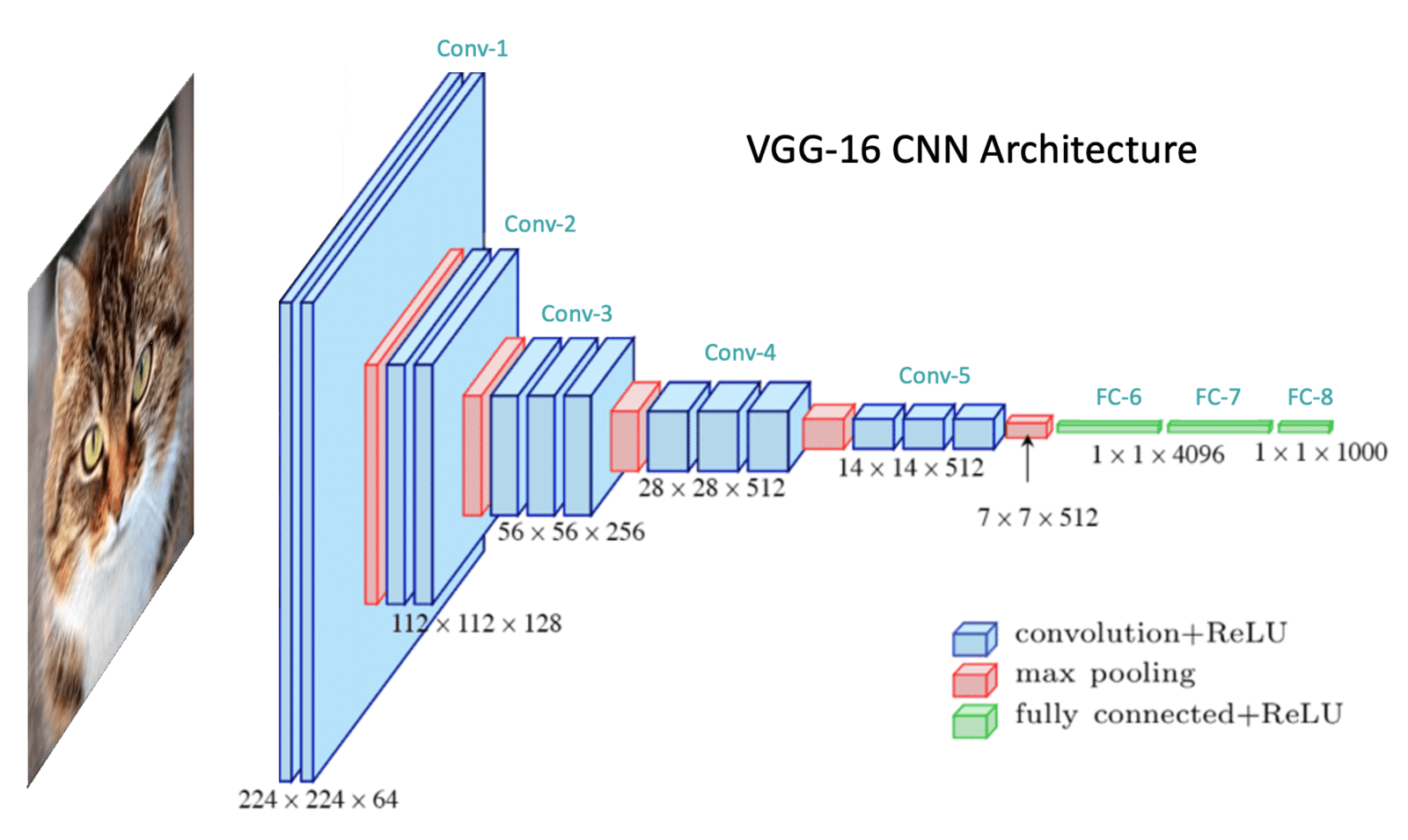
As the MIT video highlighted, this stacking creates a hierarchy of features:

• Early Layers (closer to the input) learn to detect simple features like edges, corners, and color gradients.
• Mid-level Layers combine these simple features to learn more complex patterns like eyes, noses, or textures.
• Deep Layers combine those patterns to recognize entire objects or parts of objects, like faces or car wheels.

After several convolutional blocks have successfully extracted a rich set of high-level features, the final feature maps are flattened into a single 1D vector. This vector is then fed into a standard fully-connected network (the "classifier head"), just like we studied in the previous lesson, which produces the final class probabilities (e.g., using a softmax activation function).

5. But How Are the Filters Learned?

This is perhaps the most important concept to connect back to our previous lesson. The filters are not designed by a human. The values inside the filter kernels are the weights of the network. These weights are initialized with small random numbers and are then learned automatically during the training process via backpropagation and gradient descent.

The loss function calculates the error, and backpropagation determines how to adjust the weights in every filter to make the network better at its classification task. The network itself discovers the optimal features to look for.

This short clip explains this crucial point.

For a more detailed written explanation of the entire architecture, you can refer to the following guide.

Conclusion

In this lesson, we have moved from the general-purpose, fully-connected network to the specialized architecture of the Convolutional Neural Network. You now understand the "how" behind the models that power modern computer vision.

Key Takeaways:

• Standard fully-connected networks are unsuitable for images due to parameter explosion and the loss of spatial information.
• CNNs solve this using convolution, where learnable filters (kernels) act as feature detectors that are shared across the image.
• A typical CNN architecture consists of a feature extractor and a classifier.
• The feature extractor is a series of stacked blocks, typically containing a Convolutional layer, a ReLU activation, and a Max Pooling layer.
• This structure allows the network to learn a hierarchy of features, from simple edges to complex objects.
• The final feature maps are flattened and passed to a fully-connected classifier to produce the output.
• Crucially, the filters are not hand-coded; their weights are learned via backpropagation to minimize a loss function.

Preview of the Next Lesson:

Just as CNNs are specialized for grid-like data like images, another powerful architecture has revolutionized how machines process sequential data like text. In our next lesson, we will explore the concepts of word embeddings and the Transformer architecture, which form the foundation of today's Large Language Models (LLMs).