Introduction
In our last lesson, we dissected the static architecture of a neural network, examining its core components: neurons, layers, weights, and activation functions. We established that a network is essentially a complex, parameterized function that maps inputs to outputs. The key question we left unanswered was: how does the network find the right values for its millions of parameters (weights and biases) to perform a task accurately?
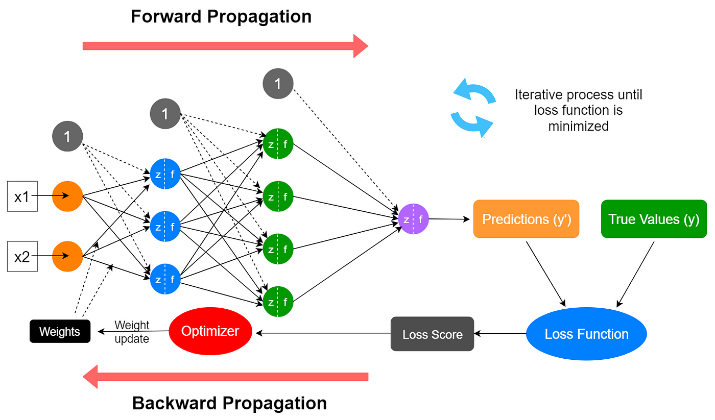
Today, we will answer that question by exploring the dynamic process of how a network learns. Our learning outcome is to explain the training loop: forward propagation for predictions, loss functions to quantify error, and backpropagation to update weights. This loop is the engine of modern machine learning, driving the process of iterative improvement that allows an AI model to go from making random guesses to performing sophisticated tasks.
The training loop consists of three fundamental steps, which we will cover in sequence:
- Forward Propagation: The network makes a prediction.
- Loss Function: The network's prediction is compared to the correct answer to quantify its error.
- Backpropagation: The error is used to calculate how to adjust the network's weights and biases to improve its next prediction.
This iterative cycle is the heart of how models are trained.
1. Forward Propagation and the Loss Function
The Forward Pass: Making a Prediction
The first step in the training loop, forward propagation, is a concept you're already familiar with from our last lesson. It's the process of passing input data through the network, from the input layer to the output layer, to generate a prediction.
At each layer, the neuron's activations are calculated by taking the weighted sum of the previous layer's activations, adding a bias, and applying an activation function. This process is repeated until the final output layer produces the network's prediction, which we often denote as ("y-hat").
The Loss Function: Quantifying Error
Once we have a prediction (), we need a way to measure how "wrong" it is compared to the actual target value (). This is the job of the loss function (or cost function). The loss function takes both the predicted and true values as input and outputs a single number—the loss—that quantifies the model's error. The goal of training is to minimize this number.
Learn to Build a Neural Network From Scratch — Yes, Really.
This article provides excellent intuition on why we need a cost function and what properties a good one should have. It explains that the core goal of machine learning is to minimize this error metric.
Please read the sections titled 'Cost intuition' and 'Cost'. Focus on these key ideas: The purpose of cost: Why do we need to quantify error? Convexity: Why is it desirable for a cost function to be 'convex' (having only one global minimum)? Binary Cross-Entropy Loss: What is the purpose of this specific loss function, which is standard for classification tasks?
As the article explains, a low cost means a good model, and a high cost means a poor one. The process of learning is simply the iterative process of adjusting the model's parameters to make the cost as low as possible.
While there are many loss functions, two common ones are:
- Mean Squared Error (MSE): Often used for regression tasks (predicting a continuous value). It is calculated as .
- Binary Cross-Entropy: Used for binary classification tasks (predicting one of two classes, e.g., 0 or 1). This function heavily penalizes confident but incorrect predictions, which makes it very effective for training classifiers.
The output of the loss function is a single number that represents the model's performance on the training data. The next step is to use this number to guide the learning process.
2. Backpropagation: The Engine of Learning
We now have a measure of the network's error. The crucial question is: how do we adjust the millions of weights and biases to reduce this error? Should we increase a particular weight? Decrease it? And by how much?
This is where backpropagation comes in. It is an algorithm that determines how much each individual weight and bias in the network contributed to the final error. It does this by propagating the error signal backward through the network, from the output layer to the input layer.
Intuition Before Calculus
Before diving into the math, it's essential to build a strong intuition for what backpropagation is doing.
Backpropagation, intuitively | Deep Learning Chapter 3
This video from 3Blue1Brown provides a brilliant and intuitive explanation of backpropagation, completely avoiding complex calculus at first. It helps build a mental model of how the algorithm works.
Watch from the beginning to 08:28. Focus on understanding the following conceptual points: How the network's error on a single training example creates a 'desired' change for the activations in the output layer. How these desired changes for one layer translate into desired changes for the layer before it (the 'backward' propagation). How the strength of a neuron's activation and the weight of its connection influence the size of the adjustment ('neurons that fire together, wire together').
As the video explains, backpropagation is fundamentally about credit (or blame) assignment. For a single training example, it calculates the "nudge" that each weight and bias should receive to steer the network's output closer to the correct answer.
This process can be visualized as descending a hill, where the hill's landscape represents the cost function. The height at any point is the cost for a given set of weights and biases. Our goal is to find the lowest point in this landscape. The algorithm that tells us which direction is "downhill" is called gradient descent. Backpropagation is the method we use to efficiently compute the gradient—a vector of partial derivatives that points in the direction of the steepest ascent. By moving in the opposite direction of the gradient, we can systematically reduce the cost.
3. The Calculus of Backpropagation
Your request for a "deep dive" into the technicals brings us to the mathematical heart of backpropagation: the chain rule from calculus. Since the cost is a function of the output layer's activations, which are themselves functions of previous layers' weights, biases, and activations, the chain rule is the tool we need to link the final error all the way back to a specific weight in an early layer.
Let's break down how (the partial derivative of the Cost with respect to a single weight ) is calculated.
Backpropagation calculus | Deep Learning Chapter 4
This follow-up video from 3Blue1Brown translates the intuition from the previous video into the formal language of calculus. It's an excellent bridge from concept to mathematics.
Watch the video up to 09:42. It will walk you through the chain of derivatives needed to find the sensitivity of the cost function to the network's parameters. Pay attention to how the chain rule links the cost (C) to an activation (a), then to a pre-activation value (z), and finally to a weight (w).
To see these calculations worked out with concrete numbers, the following article provides a detailed, step-by-step example for a very simple network.
A Comprehensive Guide to the Backpropagation Algorithm ...
This guide from Neptune.ai provides a detailed mathematical walkthrough of both the forward and backward passes. Following the numerical example will solidify your understanding of the mechanics.
Read the sections starting from 'How backpropagation algorithm works' up to the end of 'Updating weights'. You don't need to memorize the formulas, but follow the logic of how the error is calculated in the forward pass and then how the derivatives are chained together in the backward pass to update the weights.
The core idea is to compute the gradient of the cost function with respect to all parameters. This gradient, often denoted as , is a collection of all the partial derivatives ().
Once we have this gradient, we use it to update the parameters in a process called gradient descent. The update rule is simple:
Here, is the learning rate, a small hyperparameter (e.g., 0.01) that controls the size of the update step. We subtract the gradient term because the gradient points uphill, and we want to move downhill to minimize the cost. This update is performed for every weight and bias in the network.
Test your understanding!
In the gradient descent update rule, the learning rate is a critical hyperparameter. What do you think would happen if you set the learning rate too high? What if you set it too low?
Show answer
- Too high: If the learning rate is too high, the update steps will be very large. This can cause the algorithm to "overshoot" the minimum of the cost function and bounce around erratically, potentially even causing the cost to increase rather than decrease. The training process might become unstable and fail to converge.
- Too low: If the learning rate is too low, the update steps will be tiny. The model will learn, but the training process will be extremely slow, requiring many more iterations to reach the minimum. It might also get "stuck" more easily in suboptimal local minima.
This entire process—forward pass, loss calculation, backward pass, and parameter update—constitutes one step of training. This is repeated thousands or millions of times, often on small "mini-batches" of data rather than the entire dataset at once (a technique called Stochastic Gradient Descent), until the network's cost is minimized.
Conclusion
In this lesson, we have demystified the neural network training loop, the fundamental process by which AI models learn from data. You now have a deep, multi-layered understanding of this mechanism, from the high-level intuition to the underlying calculus.
Key Takeaways:
- The training process is an iterative loop of three main steps: forward propagation, loss calculation, and backpropagation.
- Forward propagation generates a prediction by passing data through the network's layers.
- A loss function (e.g., Binary Cross-Entropy) quantifies the error by comparing the network's prediction to the true value. The goal of training is to minimize this loss.
- Backpropagation is an efficient algorithm that uses the chain rule to calculate the gradient of the loss function with respect to every weight and bias in the network.
- Gradient descent uses this gradient to update the network's parameters, taking a small step in the direction that most effectively reduces the loss. The size of this step is controlled by the learning rate.
Preview of the Next Lesson:
Now that we understand the general architecture of a neural network and the universal process used to train it, we can explore specialized architectures designed for specific types of data. In the next lesson, we will focus on Convolutional Neural Networks (CNNs), the powerhouse architecture that has revolutionized computer vision by enabling machines to "see" and interpret images with remarkable accuracy.