Deriving the EM Wave Equation from Maxwell's Equations

Setting the Stage: Maxwell's Equations in a Vacuum

To begin, we need to simplify our equations for the specific environment where radar waves travel: a vacuum, or what we call "free space." In this context, "free space" is a region devoid of electric charges and electric currents.

This simplifies two of our equations:

• Since there are no charges, the charge density $\rho =0$.
• Since there are no currents, the current density $\mathbf{J}=0$.

Applying these conditions, Maxwell's four equations become:

1. Gauss's Law for $\mathbf{E}$: $\nabla \cdot \mathbf{E}=0$
2. Gauss's Law for $\mathbf{B}$: $\nabla \cdot \mathbf{B}=0$
3. Faraday's Law: $\nabla \times \mathbf{E}=-\frac{\partial \mathbf{B}}{\partial t}$
4. Ampere-Maxwell Law: $\nabla \times \mathbf{B}={\mu }_0{\epsilon }_0\frac{\partial \mathbf{E}}{\partial t}$

Notice the beautiful symmetry in the two "curl" equations (3 and 4). A change in $\mathbf{B}$ over time creates a curling $\mathbf{E}$, and a change in $\mathbf{E}$ over time creates a curling $\mathbf{B}$. This mutual induction is the engine of an electromagnetic wave.

The following video from MIT OpenCourseWare sets up this starting point and briefly reviews the key mathematical tools we'll need.

The Derivation Strategy

Our goal is to find a single equation that describes the behavior of the $\mathbf{E}$ field over space and time, without involving the $\mathbf{B}$ field. We have two coupled first-order equations (Faraday's and Ampere-Maxwell's Laws), and we want to combine them into a single second-order equation.

The strategy is as follows:

1. Take the curl of Faraday's Law ($\nabla \times \mathbf{E}=...$).
2. This will produce a term on the left, $\nabla \times (\nabla \times \mathbf{E})$, which we can simplify using the vector identity you just saw.
3. It will also produce a term on the right involving $\nabla \times \mathbf{B}$, which we can substitute using the Ampere-Maxwell Law.
4. By substituting and simplifying, we will eliminate $\mathbf{B}$ and arrive at an equation solely in terms of $\mathbf{E}$.

This process decouples the two fields, revealing the underlying wave nature of each. The following document describes this approach conceptually.

Deriving the Wave Equation for the Electric Field

Now, let's execute the derivation step-by-step. The following video and text will guide you through the mathematics. I recommend watching the video first to see the flow of the argument, then using the text to solidify your understanding of each algebraic step.

Let's formalize those steps. The following PDF presents the same derivation with mathematical rigor.

To summarize the key steps of the derivation you just studied:

1. Start with Faraday's Law:

   $$\nabla \times \mathbf{E}=-\frac{\partial \mathbf{B}}{\partial t}$$

2. Take the curl of both sides:

   $$\nabla \times (\nabla \times \mathbf{E})=\nabla \times \left(-\frac{\partial \mathbf{B}}{\partial t}\right)$$

3. Simplify the Left-Hand Side (LHS): Use the vector identity $\nabla \times (\nabla \times \mathbf{A})=\nabla (\nabla \cdot \mathbf{A})-{\nabla }^2\mathbf{A}$.

   $$\text{LHS}=\nabla (\nabla \cdot \mathbf{E})-{\nabla }^2\mathbf{E}$$

   Since we are in free space, Gauss's Law states $\nabla \cdot \mathbf{E}=0$. The first term vanishes.

   $$\text{LHS}=-{\nabla }^2\mathbf{E}$$

4. Simplify the Right-Hand Side (RHS): The space and time derivatives are independent, so we can swap their order.

   $$\text{RHS}=-\frac{\partial }{\partial t}(\nabla \times \mathbf{B})$$

   Now, substitute the Ampere-Maxwell Law for a vacuum, $\nabla \times \mathbf{B}={\mu }_0{\epsilon }_0\frac{\partial \mathbf{E}}{\partial t}$.

   $$\text{RHS}=-\frac{\partial }{\partial t}\left({\mu }_0{\epsilon }_0\frac{\partial \mathbf{E}}{\partial t}\right)=-{\mu }_0{\epsilon }_0\frac{{\partial }^2\mathbf{E}}{\partial t^2}$$

5. Equate LHS and RHS:

   $$-{\nabla }^2\mathbf{E}=-{\mu }_0{\epsilon }_0\frac{{\partial }^2\mathbf{E}}{\partial t^2}$$

   Multiplying by -1, we arrive at the 3D wave equation for the electric field:

   $${\nabla }^2\mathbf{E}={\mu }_0{\epsilon }_0\frac{{\partial }^2\mathbf{E}}{\partial t^2}$$

The Speed of Light and the Magnetic Field Wave

The general form of a 3D wave equation is ${\nabla }^{2}u=\frac{1}{v^2}\frac{{\partial }^{2}u}{\partial t^2}$, where $v$ is the speed of the wave. By comparing this to our result, we can see that the speed of our electromagnetic wave must be:

When James Clerk Maxwell first performed this calculation, the values for the permittivity of free space (${\epsilon }_0$) and the permeability of free space (${\mu }_0$) were known from tabletop electricity and magnetism experiments. Plugging in the numbers, he found that the speed of his theoretical waves was approximately $3\times 10^8$ meters per second—the measured speed of light. This was the first strong evidence that light is an electromagnetic wave. We now denote this fundamental constant as $c$.

By following an identical derivation, but starting with the Ampere-Maxwell Law and taking its curl, we can arrive at the same wave equation for the magnetic field.

So, we have two identical equations, one for $\mathbf{E}$ and one for $\mathbf{B}$:

This shows that both fields propagate in unison as a wave, traveling at the speed of light.

Visualizing the Result

The derivation shows that the interaction between changing electric and magnetic fields creates a self-sustaining wave.

The solution to the wave equation we just derived describes a traveling disturbance. As an AC current oscillates in a wire, it generates changing E and B fields. This disturbance propagates outwards, with the electric and magnetic fields constantly recreating each other as they travel.

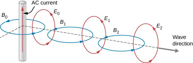
An important detail is that not just any solution to the wave equation is physically valid. The solutions must also satisfy the two divergence equations ($\nabla \cdot \mathbf{E}=0$ and $\nabla \cdot \mathbf{B}=0$). A careful analysis, which we won't detail here but is explored in the "Electromagnetic Waves Notes" resource, shows that this condition forces the waves to be transverse: both the $\mathbf{E}$ and $\mathbf{B}$ field vectors must be perpendicular to the direction of wave propagation.

Conclusion

In this lesson, you have followed the mathematical steps to derive the electromagnetic wave equation from first principles. This is a cornerstone of physics and the theoretical foundation of all radio, microwave, and radar technology.

Here are the key takeaways:

• In free space (no charges or currents), Maxwell's equations take on a highly symmetric form.
• By taking the curl of Faraday's Law and using the Ampere-Maxwell Law to substitute, we can decouple the fields and produce a second-order partial differential equation for the electric field.
• This equation is the 3D wave equation, proving that electromagnetic disturbances propagate as waves.
• The speed of these waves is determined by the fundamental constants ${\epsilon }_0$ and ${\mu }_0$, and is exactly the speed of light, $c$.
• The electric and magnetic fields propagate together, in-phase, and are perpendicular to each other and to the direction of travel, forming a transverse wave.

You now understand why electromagnetic waves exist and how their existence is a direct consequence of the fundamental laws of electricity and magnetism. In our next lesson, we will build upon this by learning how to represent these wave solutions using complex exponential notation, which provides a powerful and convenient way to describe their phase, frequency, and amplitude—the essential properties of a radar signal.