Understanding Control Flow in LLVM IR: Branches and Phis

The Challenge of Merging Paths in SSA

As you know, LLVM IR is in SSA form, meaning every virtual register is assigned a value exactly once. This simplifies many optimizations. But what happens when control flow merges? Consider a simple if-else statement where a variable x is assigned a different value in each branch. After the if-else, which value of x should be used? We can't simply re-assign x, as that would violate the single-assignment rule.

This is the central problem that control flow instructions must solve. The following video provides an excellent introduction to SSA and clearly illustrates this exact challenge.

Directing Execution with the br Instruction

The br (branch) instruction is LLVM's workhorse for directing control flow. It comes in two flavors:

1. Unconditional Branch: br label %destination
   This instruction causes an unconditional jump to the basic block identified by %destination. Every basic block must end with a "terminator" instruction, and this is the simplest one.

2. Conditional Branch: br i1 %condition, label %if_true, label %if_false
   This is how conditional logic is implemented. The first operand, %condition, must be of type i1 (a one-bit integer). If its value is 1 (true), control transfers to the %if_true block; otherwise, it transfers to the %if_false block. This %condition value is typically the result of a comparison instruction like icmp or fcmp.

Let's examine how these are used to build an if/then/else construct. The following resource walks through this exact scenario.

This structure—a conditional branch splitting the path and unconditional branches rejoining it—is the standard pattern for if-statements.

Merging Values with the phi Instruction

After reading that example, you likely noticed the phi instruction in the ifcont block. This is the solution to the problem we saw in the introductory video.

A phi instruction is a special instruction that produces a value by selecting from a list of incoming values based on which predecessor block control flowed from. Its general syntax is:

%result = phi <type> [ <value1>, <predecessor1> ], [ <value2>, <predecessor2> ], ...

In the if/then/else example from the reading:
%iftmp = phi double [ %calltmp, %then ], [ %calltmp1, %else ]

This instruction says:

• The value of %iftmp will be %calltmp if control came from the %then block.
• The value of %iftmp will be %calltmp1 if control came from the %else block.

This mechanism allows LLVM to maintain the SSA property while correctly handling values that depend on the path of execution. An important rule is that all phi instructions must appear at the very beginning of a basic block, before any non-phi instructions.

The next part of the tutorial you just read explains this in more detail.

phi Nodes vs. Stack Memory: An Optimization Perspective

You might wonder, "Why not just store the variable to a memory location on the stack in each branch and load it back after they merge?" That is indeed what happens in unoptimized builds (-O0). However, for a systems programmer concerned with performance, understanding why phi is superior is critical.

When values are kept in registers (as phi nodes allow), they are immediately available for subsequent instructions. Spilling to and reloading from the stack (alloca, store, load) introduces memory latency and prevents the optimizer from performing many analyses and transformations, such as constant propagation and instruction scheduling, as effectively. The phi node keeps the dataflow explicit and in the optimizer's direct line of sight.

The following text demonstrates this difference by comparing the IR generated with and without optimizations.

Case Study: Loops

Loops are just a specific form of control flow, and they rely on the same two instructions: br and phi. A loop is essentially a basic block (or set of blocks) that has a conditional branch at the end, which can either jump out of the loop or jump back to the beginning of the loop.

The phi node is crucial here for handling loop variables. Consider a simple for loop counter i. Its value changes on each iteration. A phi node at the start of the loop handles this perfectly:

%i.next = phi i32 [ 0, %loop.preheader ], [ %i.incremented, %loop.latch ]

This phi node initializes i to 0 when entering the loop from the preheader, and on every subsequent iteration, it takes the incremented value from the loop's back edge (the latch).

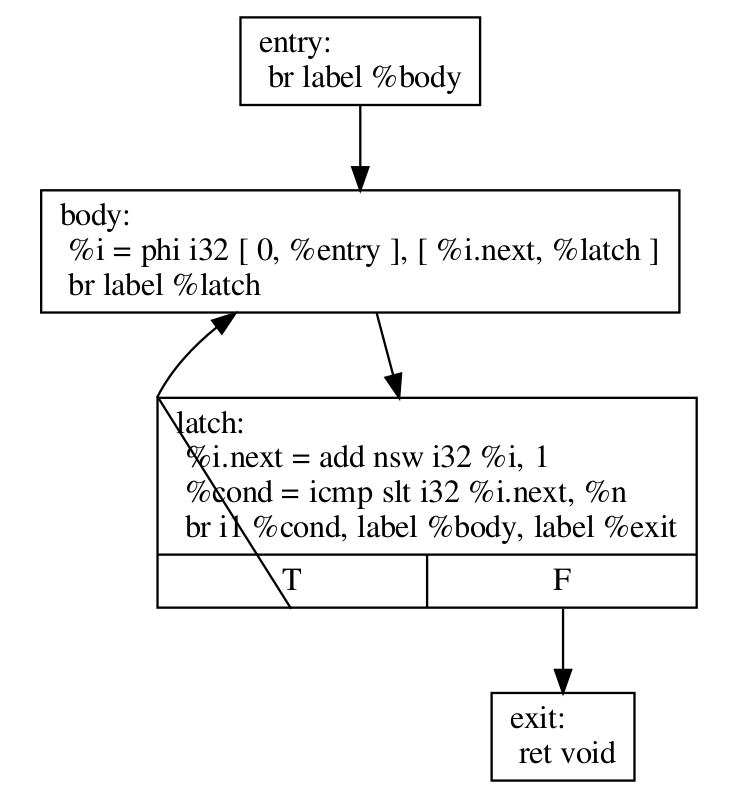
The following video segment provides a great visual walkthrough of how phi nodes enable loops.

Visualizing Control Flow: The CFG

The combination of basic blocks and the branches between them forms a directed graph called the Control Flow Graph (CFG). In a CFG, basic blocks are the nodes and the br instructions define the edges. Visualizing the CFG is an incredibly powerful way to understand a function's logic at a high level.

LLVM provides tools to do this automatically. For example, you can use opt -analyze -view-cfg your_ir_file.ll to generate and display a CFG.

Let's look at a more complex, real-world example.

By tracing the arrows and inspecting the br and phi instructions, you can reverse-engineer the entire logic of the binarySearch algorithm directly from the IR. This is a skill you will use constantly when analyzing bugs or understanding optimizer behavior.

Conclusion

In this lesson, you've learned to decode the logic of LLVM IR. You now understand the two fundamental instructions that give structure to programs: br to direct execution, and phi to merge data from different execution paths in an SSA-compliant way.

Key Takeaways:

• Terminators: Every basic block must end with a terminator instruction that transfers control, like br or ret.
• br Instruction: Comes in two forms: unconditional (br label) for simple jumps and conditional (br i1, label, label) for if-like decisions.
• phi Instruction: Solves the SSA merge problem by selecting a value based on the predecessor basic block. It is the key to representing variables whose values depend on the path taken.
• Loops: Are constructed from conditional branches that jump backward and phi nodes that manage loop-carried variables (like induction variables).
• Control Flow Graph (CFG): A visual representation of a function's logic, where basic blocks are nodes and branches are edges.

In our next lesson, we will explore metadata. While br and phi define a program's logic, metadata allows us to attach extra, non-logical information to the IR, such as source code line numbers for debugging or type information for runtime checks.