Reparameterization Trick for ELBO Optimization

Welcome to the third lesson in our exploration of the foundations of modern generative models. In our previous session, we did the heavy lifting of deriving the Evidence Lower Bound (ELBO), establishing it as a tractable proxy for the intractable log-marginal likelihood. We saw that maximizing the ELBO is equivalent to minimizing the KL divergence between our approximate posterior $q_{ϕ} (z ∣ x)$ and the true posterior $p (z ∣ x)$ .

We concluded by framing the ELBO as an objective function with two parts: a reconstruction term and a regularization term.

L (ϕ, θ) = Reconstruction Term E_{z \sim q_{ϕ} (z ∣ x)} [lo g p_{θ} (x ∣ z)] - Regularization Term D_{K L} (q_{ϕ} (z ∣ x) ∣∣ p (z))

This lesson tackles the critical "how" of optimizing this objective. The reconstruction term contains an expectation over $q_{ϕ} (z ∣ x)$ , a distribution whose parameters $ϕ$ (from the encoder) we want to optimize via gradient ascent. This presents a significant challenge: how do we calculate the gradient of an expectation with respect to the parameters of the distribution we are sampling from? The act of sampling is inherently stochastic and not a differentiable operation in the way that, for example, a matrix multiplication is.

Today, we will dissect this problem and introduce its elegant solution: the reparameterization trick. This technique is a cornerstone of variational autoencoders and many other generative models, as it makes the ELBO amenable to standard, efficient, gradient-based optimization.

The Problem: Differentiating Through a Stochastic Operation

Let's focus on the reconstruction term of the ELBO and our goal of updating the encoder parameters $ϕ$ . We need to compute the gradient:

\nabla_{ϕ} E_{z \sim q_{ϕ} (z ∣ x)} [lo g p_{θ} (x ∣ z)]

If the expectation was with respect to a fixed distribution, we could simply move the gradient operator inside the expectation. However, here the distribution $q_{ϕ} (z ∣ x)$ itself depends on $ϕ$ . This dependency introduces a complication that breaks the simple interchange of gradient and expectation.

To understand this formally, let's consider a general case from the excellent blog post "The Reparameterization Trick" by Gregory Gundersen.

The Reparameterization Trick

This article provides a formal justification for the reparameterization trick, moving beyond informal explanations. It begins by setting up the mathematical challenge we face.

Start by reading the initial sections which critique common, informal explanations. Then, carefully follow the derivation in the section "Undifferentiable expectations". This derivation, using the product rule for differentiation under the integral sign, clearly shows why an extra, problematic term appears when the distribution itself is parameterized.

As the article demonstrates, when we try to differentiate the expectation $E_{p_{θ} (z)} [f_{θ} (z)]$ with respect to $θ$ , we get two terms:

\nabla_{θ} E_{p_{θ} (z)} [f_{θ} (z)] = E_{p_{θ} (z)} [\nabla_{θ} f_{θ} (z)] + \int_{z} f_{θ} (z) \nabla_{θ} p_{θ} (z) d z

The first term, $E_{p_{θ} (z)} [\nabla_{θ} f_{θ} (z)]$ , is an expectation of a gradient, which is fine—we can estimate it with Monte Carlo sampling. The second term, however, is problematic. It is not an expectation and requires us to differentiate the probability density function $p_{θ} (z)$ itself, which is often intractable.

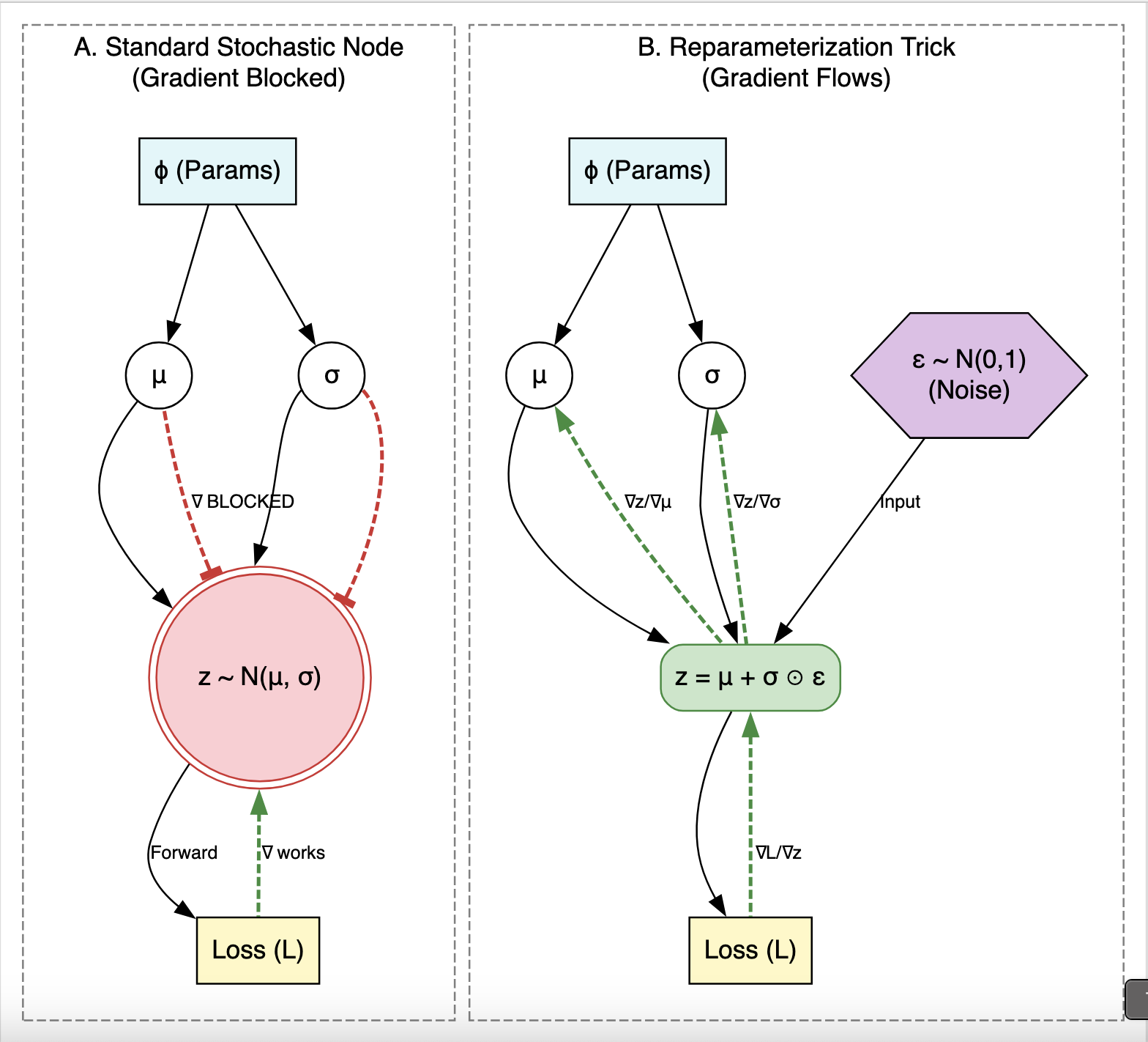
From a computational graph perspective, which you'll be familiar with from your work with PyTorch and TensorFlow, the sampling operation acts as a barrier to gradient flow. Imagine the encoder outputs parameters $μ$ and $σ$ . A subsequent "sampling node" draws $z \sim N (μ, σ)$ . The loss is calculated based on $z$ . When we use backpropagation, the gradients can't flow "backwards" through this sampling node to update $μ$ and $σ$ .

The following diagram illustrates this problem. The path for the gradient from the loss (L) to the parameters $μ$ and $σ$ is blocked by the stochastic nature of the sampling operation for $z$ .

A computational graph for a VAE. In diagram A, the standard approach shows that while the forward pass works, the gradient flow from the loss L back to the parameters $\mu$ and $\sigma$ is blocked by the stochastic sampling node $z$. In diagram B, the reparameterization trick provides a differentiable path.

The Solution: Separating Randomness from Parameters

The reparameterization trick resolves this by reframing how we generate $z$ . Instead of directly sampling from a parameterized distribution, we express $z$ as a deterministic function of its parameters and an independent, auxiliary noise variable $ϵ$ .

Let's say our approximate posterior $q_{ϕ} (z ∣ x)$ is a diagonal Gaussian, so the encoder outputs a mean vector $μ_{ϕ} (x)$ and a standard deviation vector $σ_{ϕ} (x)$ . To sample $z \sim N (μ_{ϕ} (x), diag (σ_{ϕ} (x)^{2}))$ , we can:

Sample a noise vector $ϵ$ from a fixed, standard normal distribution: $ϵ \sim N (0, I)$ .
Compute $z$ as a deterministic transformation: $z = μ_{ϕ} (x) + σ_{ϕ} (x) ⊙ ϵ$ , where $⊙$ is the element-wise product.

The random variable $z$ still has the desired distribution, $N (μ_{ϕ} (x), diag (σ_{ϕ} (x)^{2}))$ , but we have separated the source of randomness ( $ϵ$ ) from the parameters ( $μ_{ϕ}, σ_{ϕ}$ ). The stochasticity is now an input to the deterministic computation of $z$ , rather than being an operation within the graph.

This transformation is depicted in the following diagram.

This diagram illustrates the reparameterization trick. On the left, $z$ is a random node sampled from a distribution $q(z|x)$ whose parameters $\mu$ and $\sigma$ are determined by the encoder. On the right, the randomness is externalized into a fixed random node $\epsilon$, and $z$ becomes a deterministic node computed from $\mu$, $\sigma$, and $\epsilon$.

The video "Variational Autoencoder - Model, ELBO, loss function and maths explained easily!" provides a great conceptual walkthrough of this process.

Variational Autoencoder - Model, ELBO, loss function and maths explained easily!

This video explains the problem of optimizing a stochastic objective and introduces the reparameterization trick as the solution.

Watch the segment from this timestamp. It effectively describes why backpropagation fails through a stochastic sampling operation and how the reparameterization trick, by externalizing the randomness, creates a differentiable path for gradients.

Why Reparameterization Enables Gradient-Based Optimization

By reformulating $z$ , we transform the problematic gradient of an expectation into a tractable expectation of a gradient. Our original gradient was:

\nabla_{ϕ} E_{z \sim q_{ϕ} (z ∣ x)} [lo g p_{θ} (x ∣ z)]

With the trick, $z = g_{ϕ} (ϵ, x) = μ_{ϕ} (x) + σ_{ϕ} (x) ⊙ ϵ$ , and the expectation becomes:

\nabla_{ϕ} E_{ϵ \sim N (0, I)} [lo g p_{θ} (x ∣ g_{ϕ} (ϵ, x))]

Since the distribution of $ϵ$ does not depend on $ϕ$ , we can now safely move the gradient operator inside the expectation (assuming mild regularity conditions):

E_{ϵ \sim N (0, I)} [\nabla_{ϕ} lo g p_{θ} (x ∣ g_{ϕ} (ϵ, x))]

This expression is the expectation of a gradient. We can now get a low-variance, unbiased estimate of this gradient using Monte Carlo sampling. In practice, we often use a single sample of $ϵ$ per data point $x$ in a mini-batch. For one sample $ϵ^{(l)}$ , the gradient estimate is simply:

\nabla_{ϕ} lo g p_{θ} (x ∣ g_{ϕ} (ϵ^{(l)}, x))

This gradient is perfectly computable using the chain rule, which is exactly what automatic differentiation engines like autograd do. The gradient flows from the loss, through the function $lo g p_{θ}$ , through the deterministic function $g_{ϕ}$ , and back to the parameters $ϕ$ . The "gradient blocked" path in diagram A of the "Standard Stochastic Node" image is now the open path in diagram B.

The blog post "The Reparameterization Trick" formally completes this argument.

The Reparameterization Trick

This section demonstrates how the reparameterization trick transforms the gradient calculation into a form that can be estimated using Monte Carlo.

Read the section beginning with the block of equations for the reparameterized gradient. The core insight is in the step from (1) to (2), where the gradient is moved inside the expectation. Equation (3) shows the resulting Monte Carlo estimator.

This method is an instance of a pathwise derivative estimator. Its key benefit is that it typically produces gradient estimates with much lower variance than alternative methods (like the score function estimator, also known as REINFORCE), leading to more stable and faster training.

Now, let's tie this back to the full ELBO.

The Reparameterization Trick Explained

This article provides a clear summary of how the reparameterization trick fits into the optimization of the complete ELBO.

Read the section titled "Impact on ELBO Optimization". It explains that while the reconstruction term of the ELBO requires the reparameterization trick, the KL divergence term can often be computed and differentiated analytically, making the entire objective trainable end-to-end.

Conclusion

In this lesson, we have confronted a fundamental obstacle in training variational models and seen how to overcome it. We have moved from what to optimize (the ELBO) to how to optimize it.

The key takeaways are:

The gradient of an expectation with respect to the parameters of its distribution, $\nabla_{ϕ} E_{z \sim q_{ϕ}} [\cdot]$ , cannot be naively computed by moving the gradient inside.
The reparameterization trick circumvents this by expressing the random variable $z$ as a deterministic, differentiable function of its parameters ( $ϕ$ ) and an auxiliary noise variable ( $ϵ$ ) sampled from a fixed distribution.
This reformulation allows us to rewrite the gradient of the expectation as the expectation of the gradient: $E_{ϵ} [\nabla_{ϕ} \cdot]$ .
This new form can be estimated with low-variance Monte Carlo samples, and the gradient for each sample can be computed using standard backpropagation, enabling efficient, end-to-end training.

We now have all the theoretical components in place to understand how a Variational Autoencoder is trained. In our next lesson, we will synthesize these ideas to derive the complete VAE loss function as it is implemented in practice, combining the reparameterized reconstruction loss with the analytical KL divergence term. This will set the stage for our first practical implementation.

Recommended resources

The Problem: Differentiating Through a Stochastic Operation

The Solution: Separating Randomness from Parameters

Why Reparameterization Enables Gradient-Based Optimization

Conclusion