Deriving the Evidence Lower Bound (ELBO)

The Challenge: Intractable Posteriors in Latent Variable Models

Many sophisticated generative models, including VAEs, are built on the idea of latent variables. We assume that our observed data $x$ (e.g., an image) is generated by some unobserved, lower-dimensional latent variable $z$. The joint probability is given by $p(x,z)=p(x|z)p(z)$, where $p(z)$ is a prior distribution over the latents and $p(x|z)$ is the likelihood of observing $x$ given $z$.

A central task in these models is to perform inference—that is, to compute the posterior distribution of the latent variables given the data, $p(z|x)$. Using Bayes' theorem, we have:

The problem lies in the denominator, $p(x)$, known as the marginal likelihood or the evidence. It is computed by marginalizing out the latent variable:

For most interesting models, especially those with complex, high-dimensional latent spaces and nonlinear likelihood functions (like neural networks), this integral is intractable to compute. This intractability of the evidence prevents us from calculating the true posterior $p(z|x)$.

Variational Inference (VI) provides a powerful solution. Instead of computing the true posterior directly, we approximate it. We introduce a new, simpler distribution $q(z)$ from a family of tractable distributions (e.g., a Gaussian) and try to make it as close as possible to the true posterior $p(z|x)$. The "closeness" is measured, as you might guess, by the KL divergence. Our goal becomes finding the parameters of $q(z)$ that minimize $D_{KL}(q(z)||p(z|x))$. But how can we do this if we can't even compute $p(z|x)$? This is where the ELBO comes in.

A Key Mathematical Tool: Jensen's Inequality

Before we derive the ELBO, we need to introduce the mathematical tool that makes it possible: Jensen's inequality. Your background in applied mathematics will make this concept straightforward. For any convex function $f$, the line segment connecting two points on its graph lies above the graph. This generalizes to expectations.

For a convex function $f$ and a random variable $X$, Jensen's inequality states:

Since the logarithm is a concave function, the inequality is reversed:

The Stanford CS229 lecture notes on the EM algorithm provide a clear, concise explanation of this.

Deriving the Evidence Lower Bound (ELBO)

Now we have all the pieces to derive the ELBO. We will start with the intractable log-marginal likelihood, $\log p(x)$, and use a clever trick along with Jensen's inequality to find a computable lower bound.

The derivation follows these steps:

1. Start with the log-marginal likelihood, $\log p(x)$.
2. Write the marginal likelihood as an integral over the latent variable $z$.
3. Introduce our approximate distribution $q(z)$ by multiplying and dividing by it inside the integral. This is a common technique—multiplying by 1 in a creative way.
4. Recognize that the integral is now an expectation with respect to $q(z)$.
5. Apply Jensen's inequality for the concave log function to move the logarithm inside the expectation, which turns the equality into an inequality.

The same Stanford CS229 notes walk through this derivation beautifully.

Let's summarize the derivation. We start with the log evidence and introduce $q(z)$:

We can write this as an expectation with respect to $z\sim q(z)$:

Now, we apply Jensen's inequality. Since $\log$ is a concave function, we can move it inside the expectation, which flips the equality to a "greater than or equal to" sign:

The right-hand side of this inequality is the Evidence Lower Bound (ELBO). We often denote it as $\mathcal{L}(q)$ or $\text{ELBO}(q)$.

This quantity is a lower bound on the log evidence of our data. Crucially, if our choice of $q(z)$ is flexible enough and we can sample from it, we can often compute or estimate this quantity via Monte Carlo methods. This gives us a tractable objective function to optimize.

The following image provides a fantastic visual summary of this entire derivation, highlighting each key step.

The Relationship Between Evidence, ELBO, and KL Divergence

We've shown that $\log p(x)\ge \mathcal{L}(q)$. So what exactly is the gap between the true log evidence and our lower bound? It turns out to be precisely the KL divergence between our approximation $q(z)$ and the true posterior $p(z|x)$.

Let's prove this. We start with the definition of the reverse KL divergence we discussed in the last lesson:

Using Bayes' rule, we substitute $p(z|x)=\frac{p(x,z)}{p(x)}$:

Using properties of logarithms, we can split this expression:

Since $p(x)$ does not depend on $z$, the first expectation is just $\log p(x)$. The second term is exactly the negative of our ELBO definition. Therefore:

Rearranging this gives us the fundamental identity of variational inference:

This equation is profound. It tells us that the (intractable) log evidence can be decomposed into two terms: our (tractable) lower bound, the ELBO, and the (intractable) KL divergence between our approximation and the true posterior.

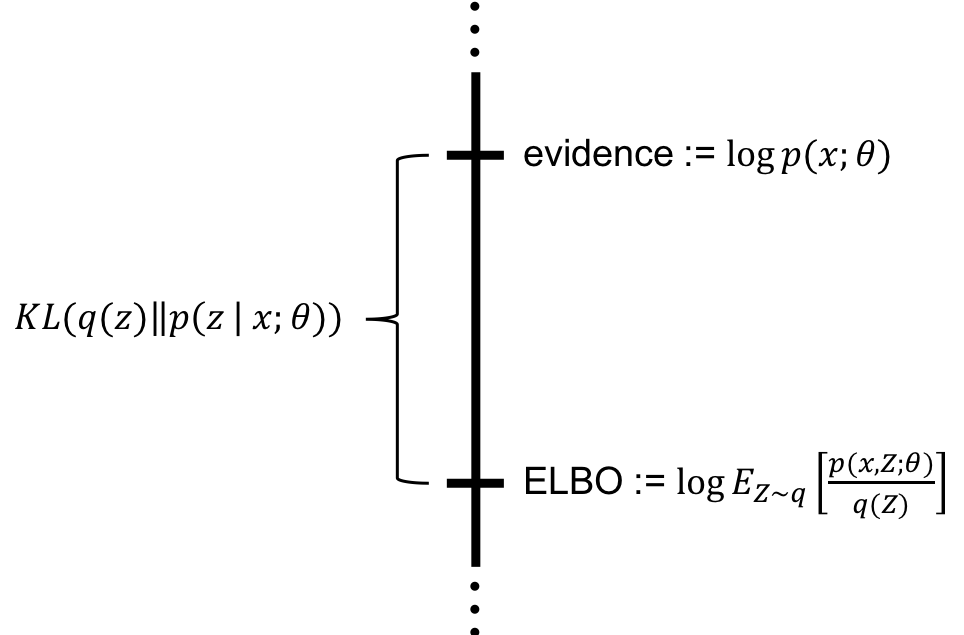
Since KL divergence is always non-negative ($D_{KL}\ge 0$), this confirms that the ELBO is indeed a lower bound on the evidence. More importantly, since the log evidence $\log p(x)$ is a fixed value for a given model and data point, maximizing the ELBO is equivalent to minimizing the KL divergence between our approximation $q(z)$ and the true posterior $p(z|x)$.

We have transformed an intractable inference problem into a tractable optimization problem. The video "Evidence Lower Bound (ELBO) - CLEARLY EXPLAINED!" provides an excellent walkthrough of this connection.

A More Practical Form of the ELBO

The ELBO can be rearranged into a more intuitive form that is widely used in practice, particularly for VAEs. We start with the definition:

Using the product rule of probability, $p(x,z)=p(x|z)p(z)$, we get:

This final expression is the one you will see most often:

This form beautifully decomposes the objective into two competing terms:

1. Reconstruction Term: ${\mathbb{E}}_{z\sim q(z)}[\log p(x|z)]$. This is the expected log-likelihood of the data, given a latent variable sampled from our approximation $q(z)$. It pushes the model to learn a $q(z)$ from which we can accurately reconstruct the original data $x$.
2. Regularization Term: $-D_{KL}(q(z)||p(z))$. This is the negative KL divergence between our approximate posterior $q(z)$ and the prior $p(z)$. It acts as a regularizer, encouraging the learned distribution of latent codes to stay close to the prior. For instance, if the prior $p(z)$ is a standard normal distribution, this term forces the approximate posteriors for all data points to cluster around the origin in the latent space.

Maximizing the ELBO now involves finding a balance between these two objectives: accurately reconstructing the data while keeping the latent representation structured and close to the prior.

Conclusion

In this lesson, we have moved from the abstract concept of KL divergence to its direct application in solving a fundamental problem in machine learning. We have rigorously derived the Evidence Lower Bound and uncovered its deep connection to the intractable marginal likelihood.

The key takeaways are:

• Variational inference addresses the problem of intractable posteriors by optimizing an approximate distribution $q(z)$.
• The Evidence Lower Bound (ELBO) is a tractable objective function derived from the log-marginal likelihood using Jensen's inequality.
• The identity $\log p(x)=\text{ELBO}+D_{KL}(q(z)||p(z|x))$ shows that maximizing the ELBO is equivalent to minimizing the KL divergence between our approximation and the true posterior.
• The ELBO can be expressed as a reconstruction term that promotes data fidelity and a KL regularization term that structures the latent space.

We have now derived what we need to optimize. In our next lesson, we will focus on how to optimize it. Specifically, we will introduce the reparameterization trick, a clever method that allows us to use standard gradient-based optimization algorithms like Stochastic Gradient Descent (SGD) to maximize the ELBO, even when it involves an expectation over a random variable.