Evaluating a Coach's Claim: Binomial Probability & Chance

Greetings, Detective. Your work on the Studio Paradox was a masterclass in navigating conflicting data. By deploying the front-door adjustment, you unmasked the truth about Velvet & Vellum's superior service, even after a key piece of evidence was deliberately "lost."

A new file has just landed on your desk, codenamed "The Coach's Miracle Cure." It concerns a charismatic relationship coach, a certain "Dr. Eve," who is making an extraordinary claim: a 100% success rate. Her marketing materials feature a dozen recent couples, all of whom, she claims, have turned their failing relationships around thanks to her revolutionary program. She presents testimonials from 12 out of 12 consecutive clients, all attesting to a significant improvement.

This is the kind of perfect record that demands scrutiny. Is Dr. Eve a miracle worker, or is she the beneficiary of an incredible lucky streak? Before we invest resources in a full-scale investigation—interviewing clients, analyzing her methods—we must first address a fundamental question: is her claim even plausible? Our first task is to determine the probability that such a perfect outcome could happen purely by chance.

Establishing a Baseline: The "Chance-Only" Hypothesis

In our last case, we compared two distinct groups. Here, we are evaluating a single claim against the backdrop of randomness. To do this, we need to establish a null hypothesis—or in our detective vernacular, a "chance-only" scenario.

Let's assume, for the sake of argument, that Dr. Eve's program has no effect whatsoever. Relationships are complex, and some couples might report improvement on their own over time, a phenomenon statisticians like yourself know can be related to regression to the mean. Let's suppose that based on broad industry data, the baseline probability of a couple reporting "significant improvement" over a similar period without any effective intervention is 50%. This gives us a benchmark for "success by chance."

Our case now boils down to this:

We have a fixed number of trials: $n = 12$ clients.
Each trial is a binary outcome: "success" or "failure."
We assume the trials are independent; one couple's outcome doesn't affect another's.
We have a constant probability of success under our chance-only hypothesis: $p = 0.5$ .

This setup perfectly describes a scenario modeled by the binomial distribution. The following video from 3Blue1Brown, though about online seller ratings, introduces this exact problem: how do we assess an underlying "success rate" based on a limited number of observations?

Binomial distributions | Probabilities of probabilities, part 1

This video provides an excellent intuitive framing for our current problem, exploring the relationship between an unknown, underlying success rate and the data we actually observe.

Watch from the beginning to see how the problem is modeled. Then, consider the core question posed from "As your first challenge...". Finally, the video provides a clear definition of the binomial distribution and when it applies.

Quantifying the Odds of a Miracle

To proceed, we need the precise mathematical tool for the job. The binomial probability mass function allows us to calculate the probability of observing exactly $k$ successes in $n$ trials.

For the binomial model to be appropriate, a few conditions must be met. The following document from NASA concisely outlines these properties.

Binomial Distribution And The “k-out-of-n” Case

This technical document provides the formal properties and formula for the binomial distribution.

Read section 3, "Properties", to confirm our case fits the model. Then, review section 4, "Formula", which gives the exact equation we need to use.

As the document states, the formula for exactly $k$ successes in $n$ trials is:

P (X = k) = (k n) p^{k} (1 - p)^{n - k}

Where $(k n) = \frac{n !}{k ! ( n - k )!}$ is the number of ways to arrange $k$ successes among $n$ trials.

In our case, we want to find the probability of Dr. Eve's perfect record: 12 successes ( $k = 12$ ) in 12 trials ( $n = 12$ ), assuming a chance-only success rate of $p = 0.5$ .

Let's plug in the numbers:

P (X = 12) = (12 12) (0.5)^{12} (1 - 0.5)^{12 - 12}

$(12 12) = \frac{12 !}{12 ! 0 !} = 1$ . There is only one way to have 12 successes in 12 trials: every single one is a success.
$(0.5)^{12}$ is the probability of 12 consecutive successes.
$(0.5)^{0} = 1$ .

So, the calculation becomes:

P (X = 12) = 1 \times (0.5)^{12} \times 1 = (\frac{1}{2})^{12} = \frac{1}{4096}

The probability is approximately $0.000244$ .

This result is our first major clue. The probability of Dr. Eve achieving a perfect 12-for-12 record purely by chance is less than 1 in 4,000. This is highly unlikely.

Interpreting the Evidence

A probability this low suggests that our initial "chance-only" hypothesis is probably wrong. While not impossible, a lucky streak of this magnitude is extremely rare.

To put this in perspective, let's consider what we would expect to see if chance were the only factor. The expected number of successes in a binomial distribution is given by $E (X) = n p$ . For our case, that would be:

E (X) = 12 \times 0.5 = 6

If the coach's method had no effect, we would expect about 6 of the 12 couples to report improvement, not all 12. The observed outcome is a huge deviation from the expected outcome.

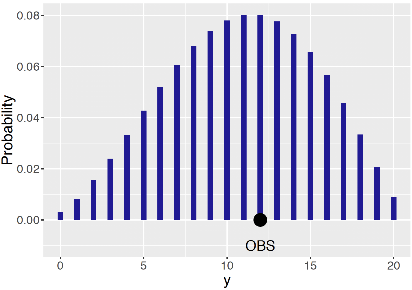
The following image illustrates this concept well. It shows a binomial probability distribution and highlights an observed value ("OBS") that is far out in the tail, just like our observation of 12 successes.

This chart shows a binomial probability distribution. Most outcomes cluster around a central value (the expected value). The point marked "OBS" represents an observed outcome that is far in the tail of the distribution, indicating it is a very rare event under this probability model. Dr. Eve's 12 successes would be a similar point on the far right of the distribution for $n=12, p=0.5$.

For a more in-depth look at applying the binomial model to test a real-world hypothesis and the derivation of the expected value, you can review the following article. It uses a baseball dataset, but the statistical reasoning is identical to ours.

Teaching the Binomial Distribution Through Baseball

This article provides a complete example of using the binomial distribution to test a hypothesis, and it includes the mathematical derivation for the expected value.

Start by reviewing the formal definition of the Binomial distribution. Then, see how it's applied in the section "Applying the Binomial Model". For completeness, you can also examine the mathematical proof in the section "Derivation of E(X)=np", which formally shows why the expected value is np.

Conclusion

Our initial forensic analysis of the numbers is complete. By applying the binomial distribution as our investigative tool, we've established that the coach's claim of a 100% success rate with 12 clients is statistically remarkable. The probability of this occurring by chance alone is minuscule ( $\approx 0.024%$ ).

This finding does not prove that Dr. Eve's method is effective, but it strongly argues against dismissing her claim as a mere fluke. We have sufficient grounds to escalate the investigation. Our work has just begun.

Key Takeaways:

A claim of a perfect success rate can be tested against a "chance-only" hypothesis using the binomial distribution.
This requires defining the number of trials ( $n$ ), the number of successes ( $k$ ), and the probability of success under the chance-only hypothesis ( $p$ ).
The binomial probability formula, $P (X = k) = (k n) p^{k} (1 - p)^{n - k}$ , quantifies the likelihood of the observed outcome.
An extremely low probability suggests that the chance-only hypothesis is not a good explanation for the data.

Preview of the Next Lesson

We've determined that something is likely happening with Dr. Eve's clients beyond simple chance. But our current analysis treats "success" as a simple binary switch. What does "success" actually mean? A tiny, barely-noticeable improvement? Or a profound, life-altering change?

In our next session, we'll dig deeper into the case files. We will analyze the paired before-and-after satisfaction scores for these clients. Our tool for this will be the sign test, a non-parametric method that will help us determine if the direction of change (improvement) is consistent and statistically significant, regardless of its magnitude.

Recommended resources

Establishing a Baseline: The "Chance-Only" Hypothesis

Quantifying the Odds of a Miracle

Interpreting the Evidence

Conclusion