Greetings, Detective.
In our last session, we confirmed that the pattern of improvement in Dr. Eve's clients was statistically significant, not just a fluke. The sign test gave us a clear signal, with a p-value of about 1.1%, allowing us to reject the idea that the program has no effect. However, by focusing only on the direction of change (up, down, or flat), we ignored a crucial part of the story: the magnitude of that change and its underlying pattern.
Today, we transition from asking if the program works to how it works. Is the improvement a fixed amount for everyone? Do couples who start with lower satisfaction see a bigger jump than those who start higher? To answer these questions, we must investigate the relationship between the Before and After scores directly. Our tools for this task are two of the most fundamental in statistics: Pearson and Spearman correlation.
The Linear Hypothesis: Pearson's Correlation
Our first line of inquiry is to test for a simple, linear relationship. Does a higher Before score correspond to a higher After score in a straight-line fashion? The standard tool for this is the Pearson correlation coefficient (). It measures the strength and direction of a linear association between two continuous variables.
Let's revisit the evidence from the 12 case files:
| Couple ID | Before Score (X) | After Score (Y) |
|---|---|---|
| 1 | 3 | 5 |
| 2 | 2 | 4 |
| 3 | 5 | 5 |
| 4 | 4 | 7 |
| 5 | 6 | 5 |
| 6 | 3 | 6 |
| 7 | 2 | 5 |
| 8 | 4 | 8 |
| 9 | 3 | 3 |
| 10 | 5 | 9 |
| 11 | 2 | 6 |
| 12 | 1 | 7 |
By applying the Pearson formula, which you'll recall is based on the covariance of the two variables scaled by their standard deviations, we get:
This value suggests a moderate, positive linear relationship. As Before scores increase, After scores also tend to increase. However, a value of 0.58 is far from a perfect +1, indicating the data points do not fall neatly on a single line. This could be due to random noise, or it could be a clue that a linear model isn't the best fit for the data.
Uncovering a Deeper Pattern: Spearman's Rank Correlation
What if the relationship isn't linear? For example, the program might provide a huge boost to couples starting with very low satisfaction, but offer diminishing returns for those already doing moderately well. This would create a relationship that is consistently increasing (monotonic) but curved, not straight.
To investigate this, we turn to Spearman's rank correlation coefficient ( or ). This non-parametric measure is a powerful tool because it assesses the relationship between the ranks of the data, not their raw values. It effectively asks: "Does a higher rank on the 'Before' scale tend to correspond with a higher rank on the 'After' scale?" This makes it robust to outliers and, crucially for our case, sensitive to monotonic relationships that are not linear.
The first step is to convert our raw scores into ranks. For each variable, the lowest score gets rank 1, the next lowest gets rank 2, and so on. When scores are tied, they all receive the average of the ranks they would have occupied.
After performing this ranking process on both the Before and After scores and then calculating the correlation on these ranks (which is mathematically equivalent to applying the Pearson formula to the ranked data), we find:
This is a significantly stronger correlation than the Pearson coefficient we calculated. This discrepancy is a major lead in our investigation.
Comparing the Evidence: Linear vs. Monotonic
We have two pieces of evidence: a Pearson of 0.58 and a Spearman of 0.71. When the Spearman correlation is notably stronger than the Pearson correlation, it's a classic sign that the underlying relationship between the variables is monotonic but not linear.
The video below from the Learn2Stats channel provides an excellent visual walkthrough of how these two coefficients behave with different data patterns.
Pearson Correlation vs Spearman Correlation (With Graph Interpretations)
This video provides a clear comparison of Pearson and Spearman correlations, highlighting their core differences with graphical examples. It will help you visualize why we might get different results from our data.
Watch the entire video, but pay special attention to the segment from the graph interpretations. This part visually demonstrates how Pearson's coefficient measures linear trends while Spearman's measures any monotonic trend, which is exactly the distinction we are exploring in Dr. Eve's data.
The images below illustrate this principle perfectly. In the top panel of each image, where the data follows a clear linear trend, the Pearson and Spearman coefficients are nearly identical. However, in the bottom panel, where the data follows a non-linear (but still increasing) curve, the Spearman coefficient is much higher than the Pearson coefficient. This is because Pearson is "penalized" by the deviation from a straight line, while Spearman only cares that as X increases, Y also consistently increases.
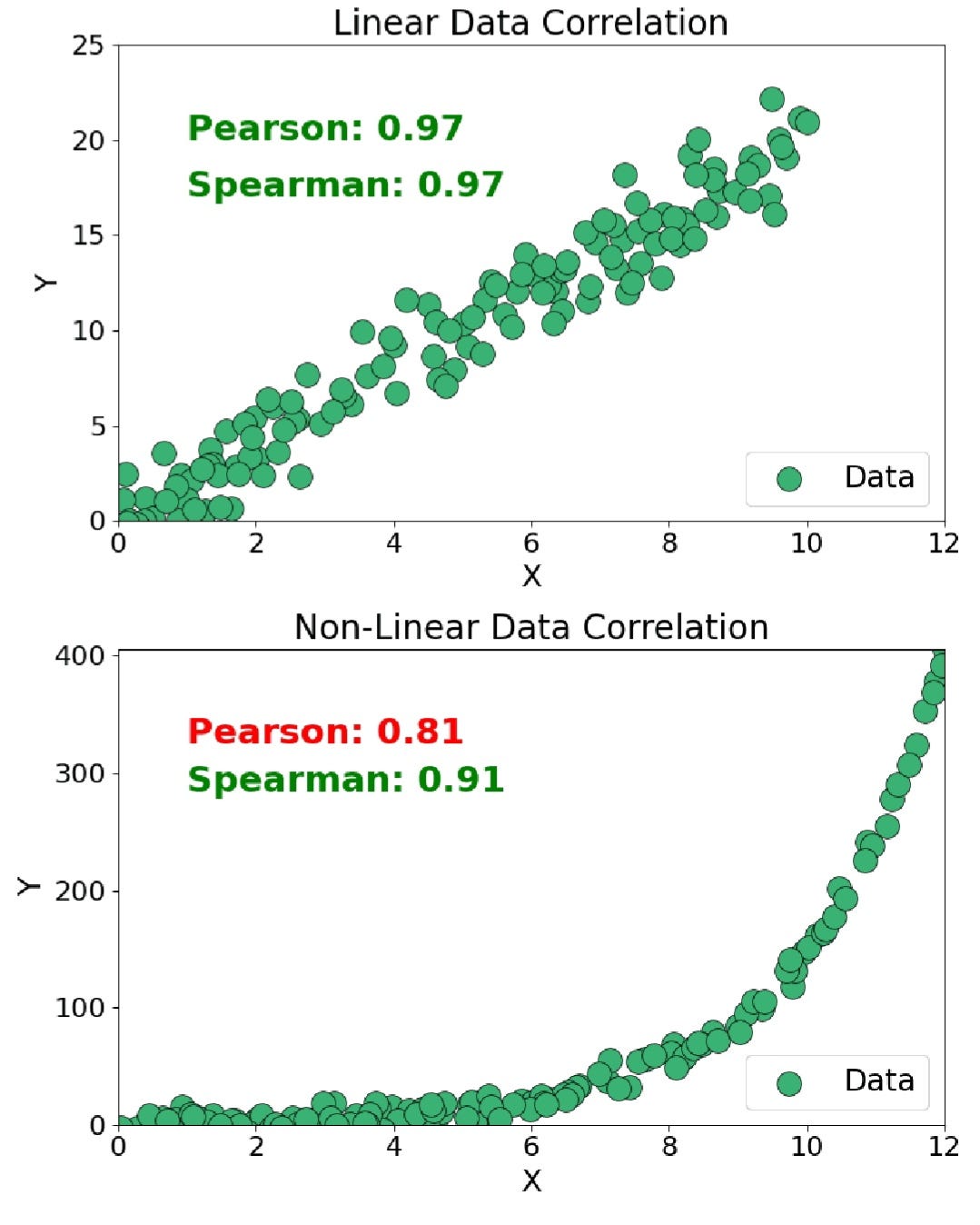
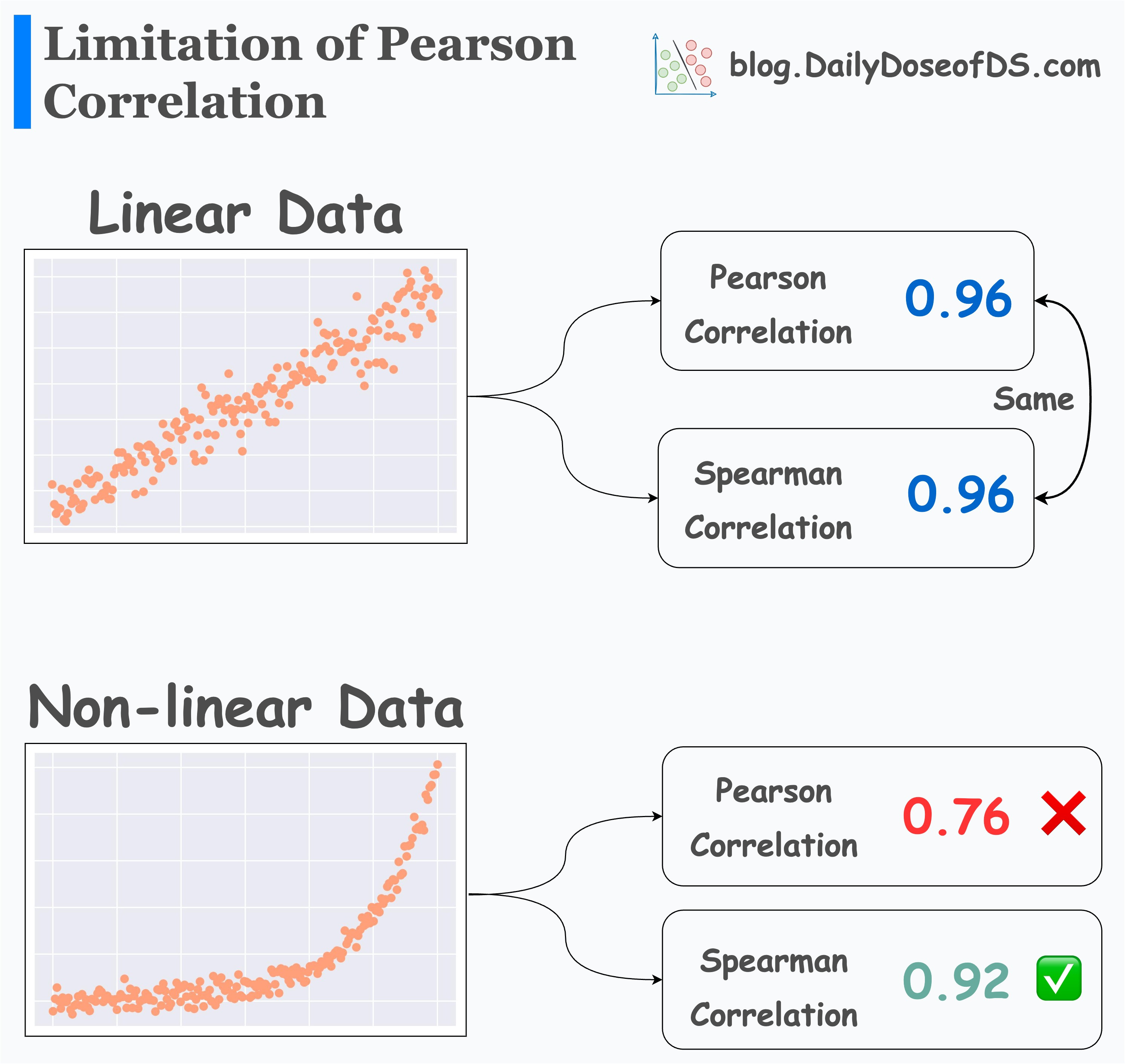
Our findings ( and ) mirror the non-linear scenarios in these exhibits. This suggests the effect of Dr. Eve's program is not a simple straight-line improvement.
To deepen our understanding of the mechanics, let's turn to some more detailed intelligence.
How to choose between Pearson and Spearman correlation?
This discussion from Cross Validated, a statistics Q&A site, offers expert insights into the distinction between these two measures. Given your background, you'll appreciate the nuance in this thread.
First, read the top answer which succinctly explains the core difference and provides a simple code example showing how S > P indicates a monotonic but non-linear relationship. Then, find the answer that discusses measurement scales, as it raises a crucial point about satisfaction scores being ordinal in nature, which is the very reason a rank-based method like Spearman's is so appropriate here.
The fact that satisfaction scores are ordinal strengthens the case for trusting the Spearman coefficient more. It doesn't assume that the interval between a score of 2 and 3 is the same as the interval between 7 and 8—an assumption that is implicit when using Pearson's .
The TileStats video below provides a step-by-step calculation of Spearman's and an excellent summary of when to use each method.
Spearman's rank correlation | Pearson VS Spearman
This video details the calculation of Spearman's correlation and provides a head-to-head comparison of its properties against Pearson's.
First, watch the segment on ranking the data, which includes an important point on handling ties. Then, focus on the final summary comparing the two methods from differences between Pearson and Spearman. This section directly addresses when each test is appropriate based on data scale (ordinal vs. continuous) and the type of relationship (linear vs. monotonic).
Conclusion
Our investigation into the relationship between Before and After scores has revealed a subtle but important pattern. While a simple linear correlation exists (), a much stronger rank-based correlation is also present (). This discrepancy is our key finding.
Key Takeaways:
- Pearson's correlation () measures the strength of a linear relationship. For our data, it was moderate.
- Spearman's correlation () measures the strength of a monotonic relationship (one that consistently moves in the same direction). For our data, it was strong.
- When , it provides strong evidence that the relationship between the variables is monotonic but non-linear.
- This suggests Dr. Eve's program does not provide a uniform, linear benefit. The effect of the program on satisfaction likely changes depending on a couple's starting point, a clue we would have missed if we had only calculated Pearson's .
Preview of the Next Lesson
We've established that the program's effect is significant and likely non-linear. But our analysis so far has been limited to just two variables: Before and After satisfaction. In the real world, client outcomes are more complex. Dr. Eve's files contain more data that she collected from her clients: their communication frequency, number of shared activities, and years together. Could these variables help us predict the final satisfaction score more accurately? Next, we will venture into the world of predictive modeling by building a multiple linear regression model to see if we can find the hidden drivers of client success—or uncover statistical evidence of something amiss.