Greetings, Detective.
The "Mystery Client" case has become a fascinating puzzle. Our initial investigation using the K-Nearest Neighbors method suggested a "Poor Fit," grouping the client with their less successful peers. Yet, when we applied the probabilistic lens of Naive Bayes, the evidence pointed to a "Successful Engagement." We are faced with two reliable methods offering contradictory conclusions. This is the classic detective's dilemma: what do you do when the forensic evidence conflicts with witness testimony?
Before we can render a final judgment, we need a third perspective—one that doesn't just give us a label, but explains its reasoning. We need a clear, logical map of the decision-making process. Today, we will construct exactly that: a two-level "decision profile" for our client. By identifying the most informative clues in their file, we will build a flowchart of questions and answers that leads to a verdict. Our goal is to create a model so transparent that it lays its logic bare for us to scrutinize.
The Art of Asking the Right Questions
Imagine you are playing "20 Questions." Your goal is to identify a secret object by asking a series of yes/no questions. A poor question like, "Is it a cuckold-themed boudoir photo album from 2021?" is too specific and will likely give you a "No," leaving you almost as uncertain as before. A good question, like "Is it a physical object?" splits the world of possibilities in half, dramatically reducing your uncertainty regardless of the answer.
This is precisely the strategy a Decision Tree employs. It seeks to find the best questions to ask about our data—the questions that most effectively split a mixed group of clients ("Successful" and "Poor Fit") into "purer," more homogeneous subgroups.
Information Gain: Formula, Calculation & Gini vs Entropy | TensorTonic
This article from TensorTonic uses the "20 Questions" analogy to build a strong intuition for how decision trees work.
Read the introduction and the analogy to solidify this core concept of asking questions that provide high information gain.
Measuring Disorder: Entropy and Gini Impurity
To find the "best" question, we first need a way to mathematically measure the "impurity" or "disorder" of a group of clients. A group with a 50/50 split of "Successful" and "Poor Fit" clients is highly impure, while a group containing only "Successful" clients is perfectly pure.
Two common measures are used for this: Entropy and the Gini Index.

-
Entropy: A concept borrowed from information theory, Entropy measures the level of uncertainty or randomness in a group. It ranges from 0 (perfectly pure) to 1 (maximum impurity, e.g., a 50/50 split). The goal of a split is to achieve the largest reduction in entropy, a quantity known as Information Gain.
-
Gini Index (or Gini Impurity): This measures the probability of incorrectly classifying a randomly chosen client from the group if it were randomly labeled according to the class distribution in that group. It ranges from 0 (perfectly pure) to 0.5 (maximum impurity). The goal is to find a split that results in the lowest weighted Gini Index for the child nodes.
In practice, both measures often produce very similar trees, but the Gini Index is computationally slightly faster as it avoids the logarithm calculation. For our detective work, understanding Gini is often sufficient.
Case File: Building the Decision Profile
Let's construct a profile using a new, more detailed client dataset. We will focus on Gini Impurity for our calculations, as it's a common default in many algorithms.
Client Data: 8 past clients, with two outcomes: "Retained" (a successful engagement) or "Lost" (a poor fit).
| Client ID | Design Aptitude (>7.5?) | Open to Experimentation? | Communication Style (Direct/Indirect) | Outcome |
|---|---|---|---|---|
| 1 | Yes | No | Direct | Retained |
| 2 | Yes | Yes | Direct | Retained |
| 3 | No | Yes | Indirect | Retained |
| 4 | No | No | Indirect | Lost |
| 5 | Yes | Yes | Indirect | Retained |
| 6 | No | Yes | Indirect | Lost |
| 7 | No | No | Direct | Lost |
| 8 | Yes | No | Indirect | Lost |
Our dataset is perfectly balanced: 4 "Retained" and 4 "Lost".
Step 1: Calculate the Gini Impurity of the Root Node
First, we calculate the impurity of the entire group. This is our baseline.
- Proportion "Retained" () = 4/8 = 0.5
- Proportion "Lost" () = 4/8 = 0.5
The Gini formula is .
This is the maximum possible Gini impurity, confirming our group is perfectly mixed.
Step 2: Evaluate Potential Splits to Find the Best Question
Now, we calculate the Gini impurity for the child nodes created by splitting on each feature. The best feature will be the one that results in the lowest weighted average Gini.
Split A: On "Design Aptitude"
- Aptitude > 7.5 (Yes): 4 clients -> 3 Retained, 1 Lost.
- Aptitude > 7.5 (No): 4 clients -> 1 Retained, 3 Lost.
- Weighted Gini (Aptitude): Since both groups have 4 clients, the weight for each is 4/8 = 0.5.
Split B: On "Open to Experimentation"
- Open = Yes: 4 clients -> 3 Retained, 1 Lost.
- Open = No: 4 clients -> 1 Retained, 3 Lost.
- Weighted Gini (Openness):
Split C: On "Communication Style"
- Style = Direct: 3 clients -> 2 Retained, 1 Lost.
- Style = Indirect: 5 clients -> 2 Retained, 3 Lost.
- Weighted Gini (Style): The weights are 3/8 and 5/8.
Decision for the Root Node:
Comparing the weighted Gini scores:
- Aptitude: 0.375
- Openness: 0.375
- Style: 0.467
The lowest Gini score is achieved by splitting on either "Design Aptitude" or "Open to Experimentation". Both are equally good first questions. Let's arbitrarily choose "Design Aptitude > 7.5?" as our root node.
This video provides a fantastic numerical walkthrough of this entire process.
Build Decision Tree using Gini Index Solved Numerical Example Machine Learning by Dr. Mahesh Huddar
This video by Dr. Mahesh Huddar shows how to build a decision tree from scratch using the Gini Index. The calculations are clear and methodical.
Watch the following segments to see the process we just performed in action: Calculating the Gini of the whole dataset. Calculating the weighted Gini for the 'Money' attribute. Calculating for the 'Parents' attribute. Calculating for the 'Weather' attribute. Comparing Gini scores to select the root node.
Step 3: Construct the Second Level of the Tree
We now have two branches from our root node. The algorithm is recursive: we repeat the exact same process for each of the new, smaller groups.
Branch 1: Clients where Aptitude > 7.5 is "No"
This group has 4 clients: 1 Retained, 3 Lost. The Gini impurity is 0.375.
The data for this subgroup is:
| Client ID | Open to Experimentation? | Communication Style | Outcome |
|---|---|---|---|
| 3 | Yes | Indirect | Retained |
| 4 | No | Indirect | Lost |
| 6 | Yes | Indirect | Lost |
| 7 | No | Direct | Lost |
We now evaluate splits on the remaining features ('Openness', 'Style') for only this group.
- Split on "Open to Experimentation":
- Open = Yes: 2 clients -> 1 Retained, 1 Lost. .
- Open = No: 2 clients -> 0 Retained, 2 Lost. Pure node! .
- Weighted Gini:
- Split on "Communication Style":
- Style = Direct: 1 client -> 0 Retained, 1 Lost. Pure node! .
- Style = Indirect: 3 clients -> 1 Retained, 2 Lost. .
- Weighted Gini:
Decision: For this branch, splitting on "Open to Experimentation" yields a lower Gini score (0.25 vs 0.334). This becomes our second-level decision.
The following resource provides an excellent demonstration of calculating splits for these subsequent, smaller nodes.
This article provides detailed calculations for building a multi-level tree. Although it uses Entropy/Information Gain, the recursive principle is identical to our Gini calculation.
Read the section "Splitting the Maths Subnode". Notice how the author takes an impure node from the first split and repeats the entire calculation process on that smaller subset of data to find the next best feature. Then, review the section on the Gini Index to see the formula and logic we've used today.
Our Final Two-Level Tree
By following this logic, we have constructed a two-level decision profile.
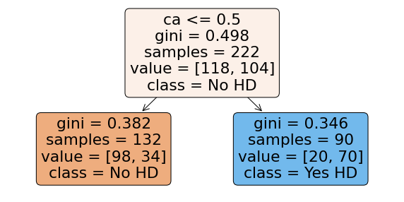
Our constructed tree would look something like this:
- Root Node: "Is Design Aptitude > 7.5?"
- If Yes: We land in a node with 3 "Retained" and 1 "Lost". We would classify a client here as Retained.
- If No: We proceed to the next question.
- Second-Level Node: "Are they Open to Experimentation?"
- If Yes: We land in a node with 1 "Retained" and 1 "Lost". The classification is ambiguous (we might default to the parent's majority or stop here).
- If No: We land in a node with 0 "Retained" and 2 "Lost". This is a pure node. We classify a client here as Lost.
Now, if our mystery client has an Aptitude Score <= 7.5 and is not open to experimentation, this model gives a clear, reasoned verdict: Lost.
Conclusion
Today, we've moved beyond black-box predictions and built a model that provides a clear, interpretable set of rules. We've seen how a decision tree, in its "greedy" quest to create the purest possible subgroups, systematically identifies the most important questions to ask. By quantifying impurity with metrics like the Gini Index, we can turn a complex dataset into a simple, powerful flowchart for classification.
Key Takeaways:
- Decision Trees create rule-based models that are highly interpretable.
- The core algorithm is recursive and greedy: at each node, it finds the single best split without looking ahead or backtracking.
- The "best" split is the one that maximizes Information Gain (reduces Entropy) or achieves the largest Gini reduction.
- Gini Impurity measures the probability of misclassification for a random element, providing a fast and effective way to evaluate splits.
- Building a tree involves calculating the impurity of the parent node and then the weighted impurity for every possible split, choosing the split that results in the greatest improvement.
Preview of the Next Lesson
We now have three verdicts on the mystery client:
- KNN: Poor Fit
- Naive Bayes: Successful Engagement
- Decision Tree: Lost (based on one possible profile)
Three different experts, three different conclusions. This is where the real detective work begins. In our final session for this case, we will act as the lead investigator. We will compare the classifications from all three models, analyze their strengths and weaknesses in this specific context, and synthesize the conflicting evidence to reach a final, definitive conclusion about the mystery client's identity and potential.