Understanding Controllability

What is Controllability?

At its core, controllability asks a simple question: "Can I get there from here?" In the context of a state-space system $\dot{\mathbf{x}}=A\mathbf{x}+B\mathbf{u}$, it asks whether the control input $\mathbf{u}(t)$ is capable of steering the state vector $\mathbf{x}(t)$ wherever we want it to go.

Let's start with a clear, conceptual definition from a video by MATLAB.

As the video explained, a system is controllable if there exists a control input $\mathbf{u}(t)$ that can transfer the system from any initial state $\mathbf{x}(t_0)$ to any final state $\mathbf{x}(t_f)$ in a finite amount of time.

This property is sometimes called reachability, and for linear systems like the ones we're studying, the two terms are used interchangeably.

To reinforce this, here is a concise written definition.

Why Controllability is the Key to Control

Defining controllability is one thing, but understanding why it's so critical is another. Controllability is not just a theoretical curiosity; it is the fundamental prerequisite for designing the controllers we'll be building.

The following video explains the profound connection between controllability and our ability to stabilize a system.

The video makes a powerful statement: A system is controllable if and only if we can arbitrarily place the eigenvalues of the closed-loop system.

Let's break this down:

1. Our open-loop system is $\dot{\mathbf{x}}=A\mathbf{x}+B\mathbf{u}$. Its stability is determined by the eigenvalues of $A$.
2. We want to design a state-feedback controller, where the control input is a linear function of the state: $\mathbf{u}=-K\mathbf{x}$.
3. Substituting this into the state equation gives the closed-loop system: $\dot{\mathbf{x}}=A\mathbf{x}+B(-K\mathbf{x})=(A-BK)\mathbf{x}$.
4. The stability of this new, controlled system is determined by the eigenvalues of the new matrix $(A-BK)$.

The fact that controllability is equivalent to "arbitrary eigenvalue placement" means that if our system is controllable, we can choose a gain matrix $K$ to place the eigenvalues of $(A-BK)$ anywhere we want.

For your inverted pendulum project, this is everything. We know the open-loop system has an unstable eigenvalue. If the system is controllable, it means we are guaranteed to be able to find a matrix $K$ that moves that unstable eigenvalue into the stable left-half plane, thereby stabilizing the pendulum. If the system were uncontrollable, there would be certain dynamics (unstable modes) that no choice of $K$ could ever fix.

The Physical Meaning of Controllability

Let's build a more physical intuition for what makes a system controllable or uncontrollable.

This car example is straightforward: if you remove the steering wheel, you lose the ability to influence the car's heading. The "heading" state is now uncontrollable. This means no matter how you use the gas and brake pedals, you cannot steer the car to a desired final state that involves a change in direction.

Now, let's consider your project, the rotary inverted pendulum.

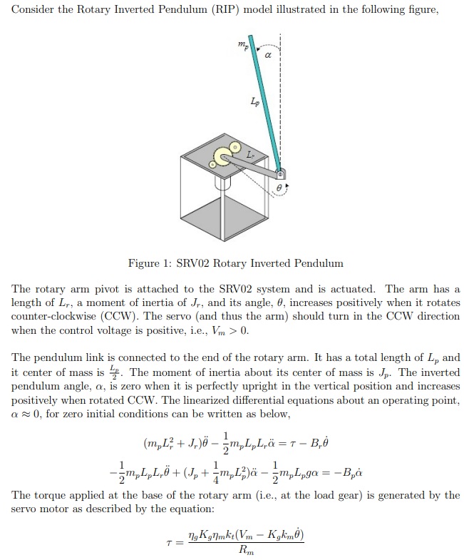
For this system, our only control input is the torque from the motor, which directly actuates the rotary arm. The question is: is this single input sufficient to control all four state variables (the position and velocity of both the arm and the pendulum)?

This is a more subtle situation. The next video clip illustrates a similar scenario where the physical configuration, not just the presence of an actuator, determines controllability. The concepts of modes and nodes from your signal processing background will be very relevant here.

The flexible beam is a fantastic example of a physical cause of uncontrollability. If an actuator is placed at a point that doesn't move for a particular vibrational mode (a node), it's physically impossible for that actuator to add or remove energy from that mode. That specific mode is therefore uncontrollable. The system as a whole is deemed uncontrollable because there's a part of its dynamic behavior that the controller can't touch.

Fortunately for us, in the rotary inverted pendulum, the dynamic coupling between the arm and the pendulum is such that actuating the arm is sufficient to influence all the states. The system is, in fact, controllable. We will prove this mathematically in our next lesson.

Conclusion

This lesson introduced the concept of controllability, a cornerstone of modern control theory.

Key Takeaways:

• Controllability is the ability to steer a system's state from any initial point to any other final point in a finite amount of time using the available control inputs.
• The physical interpretation is that our actuators must have influence over all of the system's dynamic modes. If a mode is "invisible" to the actuators (like the beam mode at a node), the system is uncontrollable.
• The primary importance of controllability is that it is the necessary and sufficient condition for being able to design a state-feedback controller that can place the closed-loop system's poles (eigenvalues) anywhere we desire. This is how we stabilize unstable systems.

Preview of the Next Lesson:

So far, we have only discussed controllability conceptually. To be useful in engineering design, we need a mathematical test. In the next lesson, you will learn how to compute the controllability matrix and use its rank to determine if a system is controllable. We will then apply this definitive test to the inverted pendulum model to prove that we can, in fact, stabilize it.