Eigenvalue Stability Analysis

The Role of Eigenvalues in System Dynamics

Let's consider a linear time-invariant (LTI) system with no input, also known as the homogeneous system:
$\dot{\mathbf{x}}(t)=A\mathbf{x}(t)$
This equation describes how the system's state evolves from an initial condition $\mathbf{x}(0)$ without any external forcing.

As an electrical engineer, you're familiar with solving linear ordinary differential equations (ODEs). The solution to this matrix ODE, $\mathbf{x}(t)$, is a combination of exponential terms in the form $e^{{\lambda }_{i}t}$, where the ${\lambda }_i$ are the eigenvalues of the matrix $A$.

The stability of the system—whether its state $\mathbf{x}(t)$ returns to the origin, blows up to infinity, or oscillates forever—depends entirely on the behavior of these $e^{{\lambda }_{i}t}$ terms as time $t\to \infty$. This is determined by the values of ${\lambda }_i$.

Stability in Continuous-Time Systems

The video below provides an excellent and intuitive explanation of how eigenvalues determine stability for both continuous and discrete-time systems.

As the video explained, the stability of a continuous-time system is determined by the real parts of the eigenvalues of the state matrix $A$.

Let's summarize the rules:

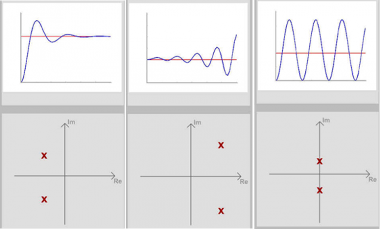
• Asymptotic Stability: The system is asymptotically stable if and only if all eigenvalues of $A$ have negative real parts ($\text{Re}({\lambda }_i)<0$). This means any initial perturbation will decay to zero over time.
• Instability: The system is unstable if at least one eigenvalue of $A$ has a positive real part ($\text{Re}({\lambda }_i)>0$). This means a small perturbation will cause the state to grow without bound.
• Marginal Stability: The system is marginally stable if it is not unstable, but at least one eigenvalue has a zero real part ($\text{Re}({\lambda }_i)=0$). This typically results in sustained oscillations (for $\lambda =\pm j\omega$) or a constant offset (for $\lambda =0$).

This concept is often visualized using the complex s-plane, which should be familiar from your work with transfer functions.

For a more formal definition and a practical example, let's turn to a concise reading.

The inverted pendulum example is particularly insightful. The analysis shows that its linearized A matrix will always have a positive real eigenvalue, mathematically proving that the upright position is inherently unstable. Our goal in later lessons will be to design a feedback controller that moves this unstable eigenvalue into the stable left half-plane.

The Eigenvalue-Pole Equivalence

As we've been emphasizing, the stability rules for eigenvalues are identical to the stability rules for poles. This is no coincidence. The following short video reinforces the direct mathematical link we discovered in the last lesson.

This confirms that whether you're working with transfer functions or state-space models, you're analyzing the same fundamental system property.

Stability in Discrete-Time Systems

While most of your experience is with continuous-time systems, modern control is often implemented on digital computers, which operate in discrete time steps. It's useful to know how the stability criterion changes in this context.

A discrete-time LTI system is described by:
$\mathbf{x}[k+1]=A_d\mathbf{x}[k]$
Here, the state at the next time step, $k+1$, is found by multiplying the current state by the matrix $A_d$. The solution involves terms of the form ${\lambda }^k$.

To summarize the discrete-time stability rules:

• Asymptotic Stability: The system is asymptotically stable if and only if all eigenvalues of $A_d$ have a magnitude less than 1 ($|{\lambda }_i|<1$).
• Instability: The system is unstable if at least one eigenvalue has a magnitude greater than 1 ($|{\lambda }_i|>1$).
• Marginal Stability: The system is marginally stable if it is not unstable, but at least one eigenvalue has a magnitude equal to 1 ($|{\lambda }_i|=1$).

This distinction is crucial when you move from designing a controller in the continuous domain to implementing it on a microcontroller.

Conclusion

In this lesson, we have established a clear and powerful method for analyzing system stability directly from the state-space representation.

Key Takeaways:

• The stability of an LTI system is determined by the eigenvalues of its state matrix $A$.
• For a continuous-time system ($\dot{\mathbf{x}}=A\mathbf{x}$), it is asymptotically stable if all eigenvalues lie in the left half of the complex plane ($\text{Re}({\lambda }_i)<0$).
• For a discrete-time system ($\mathbf{x}[k+1]=A_d\mathbf{x}[k]$), it is asymptotically stable if all eigenvalues lie inside the unit circle ($|{\lambda }_i|<1$).
• This analysis confirms that an inverted pendulum is inherently unstable, as it possesses an eigenvalue in the right half-plane.

Preview of the Next Lesson:

Knowing a system is unstable is the first step. The next logical question is: can we stabilize it? The ability to influence a system's states through its inputs is a fundamental property called controllability. In our next lesson, we will define controllability and learn how to determine if a system is controllable, setting the stage for controller design.