State-Space Modeling of a Rotary Inverted Pendulum

The System: A Rotary Inverted Pendulum

First, let's get a clear picture of the physical system we're dealing with.

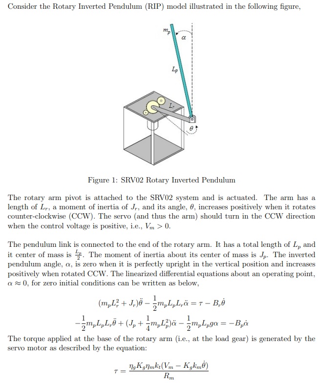
As shown, the key components are:

• A servo motor that applies a torque to a rotary arm.
• A rotary arm of length $r$ that rotates horizontally. Its angle is denoted by $\theta$.
• A pendulum of length $L$ and mass $m$ attached to the end of the arm. Its angle relative to the vertical is $\alpha$.

Our control input will be the voltage applied to the motor, and the variables we want to control are the angles $\theta$ and $\alpha$.

Modeling Strategy

Deriving the model from first principles is a multi-step process:

1. Mechanical Model: We'll start by applying physical laws (like Euler-Lagrange) to the arm and pendulum to get a set of coupled, nonlinear differential equations describing their motion.
2. Electrical Model: We will then model the DC motor to find the relationship between the applied voltage (our actual input, $V$) and the torque ($T$) it produces. This step is crucial for a realistic model and connects directly to your background in electrical engineering.
3. Combine and Linearize: We'll combine the electrical and mechanical models and then linearize the resulting nonlinear equations around the desired operating point (i.e., the pendulum balanced upright).
4. State-Space Formulation: Finally, we'll arrange these linearized equations into the standard MIMO state-space form: $\dot{\mathbf{x}}=A\mathbf{x}+B\mathbf{u}$.

The following resource provides a step-by-step derivation that follows this exact strategy.

Deconstructing the Model Derivation

Let's summarize the key stages from the document you just read.

1. Nonlinear Equations of Motion

The document uses the Euler-Lagrange method to arrive at two coupled, second-order nonlinear differential equations.

• Equation (5) describes the motion of the rotary arm ($\theta$): $$(J_{eq}+m{r}^2)\ddot{\theta }-(mLr)\cos (\alpha )\ddot{\alpha }+(mLr)\sin (\alpha ){\dot{\alpha }}^2+B_{eq}\dot{\theta }=T$$
• Equation (6) describes the motion of the pendulum ($\alpha$): $$\frac{4}{3}m{L}^2\ddot{\alpha }-(mLr)\cos (\alpha )\ddot{\theta }-(mgL)\sin (\alpha )=0$$

Notice the coupling terms like $\cos (\alpha )\ddot{\theta }$ and $\cos (\alpha )\ddot{\alpha }$. These show that the motion of the arm affects the pendulum and vice-versa. The presence of trigonometric functions ($\sin (\alpha ),\cos (\alpha )$) and squared velocity terms (${\dot{\alpha }}^2$) makes these equations nonlinear.

2. The Motor Model

Section 2.1.2 introduces the DC motor equations. For our purposes, the most important result is Equation (7), which gives the generated torque $T$ as a function of the input voltage $V$ and the arm's angular velocity $\dot{\theta }$:

This equation shows that the torque isn't just proportional to voltage; there's also a "back-EMF" damping effect proportional to the motor's speed. By substituting this expression for $T$ into the mechanical equations, we can describe the entire system's dynamics in terms of the voltage input $V$.

3. Linearization and State-Space Formulation

To use linear control techniques, we must linearize the model around the unstable equilibrium point: $\alpha =0$ (pendulum upright and not moving). For small deviations around this point:

• $\sin (\alpha )\approx \alpha$
• $\cos (\alpha )\approx 1$
• Terms like ${\dot{\alpha }}^2$ are considered negligible.

Applying these approximations to the combined electro-mechanical equations yields a set of linear differential equations. The final step is to define the state vector and arrange these equations into matrix form.

A logical choice for the state variables, stemming from the two second-order differential equations, is the angles and their velocities:

With this state vector, the input $u=V$, and the definitions of the constants $a,b,c,d,E,G$ from the resource, the system can be written as:

The first two rows are simply the definitions $\dot{\theta }=\dot{\theta }$ and $\dot{\alpha }=\dot{\alpha }$. The last two rows contain the complex dynamics derived from the linearized physics. This is our complete linear state-space model for the rotary inverted pendulum.

Another very similar derivation is presented in the resource "EE-479 Digital Control System Project 3 Rotary Inverted ...", which you can use as an alternative reference. It uses slightly different notation but arrives at the same underlying model structure (see Equation 3.23 in that document).

Conclusion

In this lesson, you have taken a significant step toward your goal by deriving a complete, linearized state-space model for the rotary inverted pendulum. This process integrated concepts from physics, electrical engineering, and control theory.

Key Takeaways:

• Modeling a complex electro-mechanical system involves deriving equations for both its mechanical and electrical components.
• The dynamics of the rotary inverted pendulum are inherently nonlinear and coupled.
• Linearization around an equilibrium point (even an unstable one) allows us to create a linear model suitable for standard control design techniques.
• The final state-space model consists of a 4x4 $A$ matrix and a 4x1 $B$ matrix, representing a system with 4 state variables and 1 control input (voltage).

Preview of the Next Lesson:
Now that we have the state-space model $(A,B,C,D)$, what does it tell us about the system's behavior? In the next lesson, we will derive the transfer function matrix from this MIMO state-space representation. This will give us a frequency-domain perspective, helping us understand how the motor voltage input influences the arm and pendulum angles, and will reveal important properties of the system.