MIMO System Controllability and Observability Analysis

Part 1: Controllability

Controllability addresses whether it's possible to steer a system from any initial state to any desired final state within a finite time, using the available control inputs.

For your inverted pendulum project, this asks: "Can we use the motor voltage to arbitrarily control the four states: arm angle $\theta$, pendulum angle $\alpha$, and their velocities $\dot{\theta }$ and $\dot{\alpha }$?" If the answer is no, then no matter how sophisticated our controller is, there will be parts of the system's behavior we simply cannot command.

The Controllability Test

To check for controllability, we construct the Controllability Matrix, often denoted as $\mathcal{C}$. For a system with $n$ state variables, this matrix is formed by combining the influence of the input matrix $B$ over time.

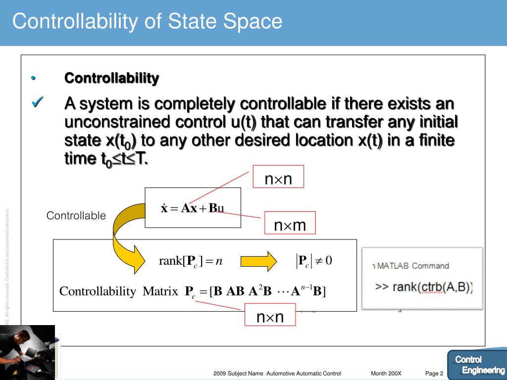
The matrix is constructed as follows:

The system is controllable if and only if this matrix has full rank, meaning:

Intuitively, if the rank is less than $n$, it means the control input cannot influence the states in certain "directions" of the state-space. The system has uncontrollable modes.

Practical Analysis with MATLAB

Calculating this matrix and its rank by hand is tedious. In practice, we use computational tools. The following video demonstrates this using the inverted pendulum on a cart, a system very similar to your own. It clearly shows how to use MATLAB to determine if the system is controllable.

As the video showed, the process in MATLAB is very direct:

% Assume A and B are your state-space matrices for the pendulum
Co = ctrb(A, B);  % 'Co' for Controllability matrix
rank_Co = rank(Co);

% If rank_Co equals the number of states (4 for our pendulum), 
% the system is controllable.

For a more detailed textual reference on this topic, the following resource is excellent. It formally defines the controllability matrix and shows the same MATLAB implementation.

Part 2: Observability

Observability is the dual concept to controllability. It addresses whether we can determine the complete internal state vector $\mathbf{x}$ by observing the system's outputs $\mathbf{y}$ over a finite period.

For your project, this asks: "If our sensors can only measure the angles $\theta$ and $\alpha$, can we use that information to calculate the angular velocities $\dot{\theta }$ and $\dot{\alpha }$?" If a system is not observable, some states are "hidden" from our sensors, and we cannot build a state-estimator (like an observer) to reconstruct them. This has major implications for control, as many advanced techniques require access to the full state vector.

The Observability Test

To check for observability, we construct the Observability Matrix, $\mathcal{O}$.

The matrix is constructed as:

The system is observable if and only if this matrix has full rank:

Given your background in signal processing, you can think of this as a signal reconstruction problem. Is the output signal $\mathbf{y}(t)$ rich enough to uniquely reconstruct the internal state signal $\mathbf{x}(t)$? If the rank is less than $n$, some state dynamics produce no effect on the output, making them impossible to observe.

Practical Analysis and the Importance of Sensor Choice

The choice of sensors (which defines the $C$ matrix) is critical for observability. A system might be observable with one set of measurements but unobservable with another.

The following video is an excellent practical demonstration of this. It shows how changing the output matrix $C$ for the inverted pendulum directly impacts observability.

This video provides a crucial insight: simply measuring the pendulum's angle is not enough to determine the cart's absolute position, because the system dynamics are independent of that absolute position (they are translationally invariant). This makes the state associated with the cart's position unobservable from an angle-only measurement.

The MATLAB process is, again, very straightforward:

% Assume A and C are your state-space matrices
Ob = obsv(A, C);  % 'Ob' for Observability matrix
rank_Ob = rank(Ob);

% If rank_Ob equals the number of states, the system is observable.

The CTMS page you looked at earlier also covers observability right after controllability, providing a good textual summary.

Conclusion

In this lesson, you've learned how to perform one of the most fundamental analyses in control theory. These checks are a mandatory first step before attempting to design a state-feedback controller or a state observer.

Key Takeaways:

• Controllability determines if the inputs can steer the system to any desired state. It is tested by checking if $\text{rank}(\mathcal{C})=n$, where $\mathcal{C}=\text{ctrb}(A,B)$.
• Observability determines if the internal states can be deduced from the system's outputs. It is tested by checking if $\text{rank}(\mathcal{O})=n$, where $\mathcal{O}=\text{obsv}(A,C)$.
• These properties are inherent to the system model ($A,B,C$ matrices) and are prerequisites for designing effective controllers and estimators.

Preview of the Next Lesson:
We've established that the inverted pendulum system is indeed controllable and observable (with the right sensors). Now we can proceed. In the previous lesson, you learned how to find the transfer function matrix $G(s)$. Our next lesson will focus on using this matrix to identify coupling between different input-output channels. This will help us understand how, for example, a command to control the arm angle might undesirably affect the pendulum angle, and vice-versa.